Next: Bibliography Up: Linear Tearing Mode Stability Previous: Resonant Layer Thickness Contents
 |
 |
(6.29) |
 |
 |
(6.30) |
 is bounded as
 , and
as
, and
as
 . Here, use has been made of Equations (6.8), (6.26), and (6.27).
As is easily demonstrated (see Section 5.14), the solution of Equation (6.28) that is bounded as
is
where
. Here, use has been made of Equations (6.8), (6.26), and (6.27).
As is easily demonstrated (see Section 5.14), the solution of Equation (6.28) that is bounded as
is
where
 |
(6.36) |
 is an arbitrary constant.
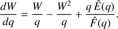
Let us again (see Section 5.14) make the Riccati transformation [2,5]
 |
(6.37) |
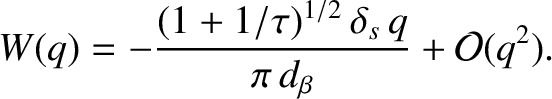
 behavior of the solution to the previous equation is
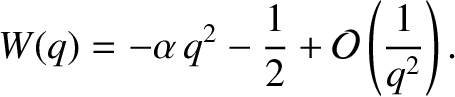
Likewise, according to Equation (6.35), the large- behavior of the solution is
Equation (6.38) is conveniently solved numerically by launching a solution of the form (6.40) at large , and then
integrating backward to small [5]. It follows from Equation (6.39) that
behavior of the solution to the previous equation is
Likewise, according to Equation (6.35), the large- behavior of the solution is
Equation (6.38) is conveniently solved numerically by launching a solution of the form (6.40) at large , and then
integrating backward to small [5]. It follows from Equation (6.39) that
![$\displaystyle \frac{\delta_s}{d_\beta}= -\lim_{q\rightarrow 0}\left[\frac{\pi}{(1+1/\tau)^{1/2}}\,\frac{dW}{dq}\right].$](img2476.png) |
(6.41) |
Table 6.2 gives estimates for the normalized resonant layer parameters,
 ,
,
 ,
and
,
and
 , that appear in Equations (6.28)–(6.30), in a low-field and a high-field tokamak fusion reactor. These estimates are made using the
data shown in Table 6.1. Table 6.2 also gives estimates for the linear layer thicknesses and tearing mode growth-rates in such reactors. These estimates are obtained via numerical solution of the resonant layer equation.
It can be seen that the typical radial thickness of a
linear tearing layer in a tokamak fusion reactor is only a few millimeters. Furthermore,
linear tearing modes in tokamak fusion reactors grow on timescales that typically lie between a tenth of a second and a second [assuming that
, that appear in Equations (6.28)–(6.30), in a low-field and a high-field tokamak fusion reactor. These estimates are made using the
data shown in Table 6.1. Table 6.2 also gives estimates for the linear layer thicknesses and tearing mode growth-rates in such reactors. These estimates are obtained via numerical solution of the resonant layer equation.
It can be seen that the typical radial thickness of a
linear tearing layer in a tokamak fusion reactor is only a few millimeters. Furthermore,
linear tearing modes in tokamak fusion reactors grow on timescales that typically lie between a tenth of a second and a second [assuming that
 .]
Finally, the real frequencies of such modes, in a frame of reference that co-rotates with the electron fluid
at the resonant surface, (i.e., the imaginary components of
.]
Finally, the real frequencies of such modes, in a frame of reference that co-rotates with the electron fluid
at the resonant surface, (i.e., the imaginary components of  ) are very much smaller (by a factor of order
  ) than a typical diamagnetic frequency. (See Table 6.1.) In other words, linear tearing modes do indeed co-rotate with the electron
fluid at the resonant surface to a very high degree of fidelity.
) than a typical diamagnetic frequency. (See Table 6.1.) In other words, linear tearing modes do indeed co-rotate with the electron
fluid at the resonant surface to a very high degree of fidelity.
Figures 6.2 and 6.3 show values of
 and
and
 , respectively, evaluated numerically as functions of
and
, respectively, evaluated numerically as functions of
and
 . In producing these figures, it is assumed that
 . The fact that
 for all values of
and confirms that tearing modes are linearly unstable for
for all values of
and confirms that tearing modes are linearly unstable for  , and stable otherwise [4]. [See Equation (6.25).] It is clear that the layer width increases with increasing normalized
diamagnetic frequency,
, and also with increasing normalized magnetic Prandtl number, .
, and stable otherwise [4]. [See Equation (6.25).] It is clear that the layer width increases with increasing normalized
diamagnetic frequency,
, and also with increasing normalized magnetic Prandtl number, .


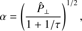
![$\displaystyle Y_e(q) = Y_0\left[1- \frac{(1+1/\tau)^{1/2}\,\delta_s\,q}{\pi\,d_\beta} + {\cal O}(q^2)\right]$](img2465.png)
![$\displaystyle Y_e(q) = \frac{A\,{\rm e}^{-\alpha\,q^2/2}}{q^{1/2}}\left[1+{\cal O}\left(\frac{1}{q^2}\right)\right],$](img2467.png)

![\includegraphics[width=1.\textwidth]{Chapter06/Figure6_2.eps}](img2471.png)
![\includegraphics[width=1.\textwidth]{Chapter06/Figure6_3.eps}](img2477.png)