Determination of Linear Growth-Rates

Reusing the analysis of Sections 5.7–5.9, let us again suppose that there are two layers in $p$ space (i.e., Fourier space). The small-$p$ layer turns out to be of width $\vert\hat{\gamma}\vert^{1/2}$, where

$$\hat{\gamma} = S^{1/3}\,\gamma\,\tau_H.$$ (6.4)

Here, $\tau _H$ is the hydromagnetic timescale defined in Equation (5.43). Given that we are effectively assuming that $\vert\hat{\gamma}\vert\ll 1$, the condition for the separation of the layer solution into two layers (i.e., that the width of the small-$p$ layer is less than that of the large-$p$ layer) is always satisfied. The large-$p$ layer is governed by the equation

$$\frac{d^2 Y_e}{dp^2} - \frac{E(p)}{F(p)} \,Y_e =0,$$ (6.5)

where

$$E(p) \simeq -(1+1/\tau)^{-1}\,Q_\ast^{\,2} -{\rm i}\,Q_\ast\,(P_\varphi+P_\perp)\,p^2+ P_\varphi\,P_\perp\,p^4,$$ (6.6)

$$F(p) \simeq P_\perp - {\rm i}\,Q_\ast\,D^2 +(1+1/\tau)\,P_\varphi\,D^2\,p^2.$$ (6.7)

Here, $Q_\ast$ is the normalized diamagnetic frequency [see Equation (5.65)], $P_\varphi$ and $P_\perp$ are magnetic Prandtl numbers [see Equations (5.53) and (5.54)], and $\tau$ is the ratio of the electron to the ion pressure gradient at the rational surface [see Equation (4.5)]. The boundary conditions on Equation (6.5) are that $Y_e$ is bounded as $p\rightarrow\infty$, and

$$Y_e(p)= Y_0\left[1-\frac{\skew{6}\hat{\mit\Delta}\,p}{\pi\,\hat{\gamma}} + {\cal O}(p^2)\right]$$ (6.8)

as $p\rightarrow 0$. Here, $Y_0$ is an arbitrary constant.

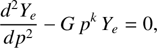
In the various constant-$\psi$ linear growth-rate regimes considered in the next section, Equation (6.5) reduces to an equation of the form

$$\frac{d^2 Y_e}{dp^2} - G\,p^k\,Y_e = 0,$$ (6.9)

where $k$ is real and non-negative, and $G$ is a complex constant. As described in Section 5.8, the solution of this equation that is bounded as $p\rightarrow\infty$ can be matched to the small-$p$ asymptotic form (6.8) to give

$$\skew{6}\hat{\mit\Delta} =\frac{ \nu^{2\nu-1}\,\pi\,{\mit\Gamma}(1-\nu)}{{\mit\Gamma}(\nu)}\,G^{\,\nu}\,\hat{\gamma},$$ (6.10)

where $\nu=1/(k+2)$. The width of the large-$p$ layer in $p$ space is $\vert G\vert^{-\nu}$.