Next: Plasma Equilibrium Up: Linear Resonant Response Model Previous: Introduction Contents
 , (see Section 4.3) in our reduced drift-MHD model equal to the minor radius of the rational surface,
  . The model evolves four scalar fields. These fields are the (normalized) helical magnetic flux,
  , the (normalized) perturbed total plasma pressure,
  , the (normalized)
MHD fluid stream-function,
, the (normalized)
MHD fluid stream-function,  , and the (normalized) ion
parallel velocity,
, and the (normalized) ion
parallel velocity,  . Our four fields have the following definitions:
where
. Our four fields have the following definitions:
where
 |
 |
(5.5) |
 |
 |
(5.6) |
 |
 |
(5.7) |
 ,
,  ,
,  are conventional cylindrical coordinates,
 ,
,
 ,
,
 ,
,
 a helical angle,
 a simulated toroidal angle (see Chapter 3),
 the magnetic field-strength,
  the (spatially constant) equilibrium magnetic
field-strength,
the (spatially constant) equilibrium magnetic
field-strength,  the Alfvén speed [see Equation (4.23)],
  the MHD fluid velocity [see Equation (2.321)],
  the collisionless ion skin-depth [see Equation (4.24)],
 ,
,
 the total plasma pressure,
  the equilibrium total plasma pressure at the rational surface,
  the
safety-factor profile, and
the
safety-factor profile, and  the simulated major radius of the plasma.
The reduced drift-MHD response model also employs the auxiliary fields
the simulated major radius of the plasma.
The reduced drift-MHD response model also employs the auxiliary fields
 |
 |
(5.8) |
 |
 |
(5.9) |
 .
.
The reduced drift-MHD model takes the form (see Section 4.5)
Here,![$[A,B]\equiv \hat{\nabla}A\times \hat{\nabla}B\cdot{\bf n}$](img1984.png) ,
,
 is the (normalized) parallel inductive electric field that maintains the parallel plasma current at the rational surface against ohmic decay,
  the ratio of the electron to the ion equilibrium pressure gradient at the rational surface [see Equation (4.5)],
  a dimensionless measure of the plasma pressure at the rational surface [see Equation (4.65)],
 the ion sound radius at the rational surface, and
 . Finally,
 |
 |
(5.14) |
 |
 |
(5.15) |
 |
![$\displaystyle = \frac{2}{3}\left(\frac{1-c_\beta^2}{r_s\,V_A}\right)\left[\left...
...tau}\right)\left(\frac{\eta_i}{1+\eta_i}\right)\chi_{\parallel\,i}(r_s)\right],$](img1994.png) |
(5.16) |
 |
![$\displaystyle = \frac{2}{3}\left(\frac{1-c_\beta^2}{r_s\,V_A}\right)\left[\left...
...{1+\tau}\right)\left(\frac{\eta_i}{1+\eta_i}\right)\chi_{\perp\,i}(r_s)\right].$](img1996.png) |
(5.17) |
 and
and  are defined in
Equations (4.3) and (4.4), respectively. Moreover,
are defined in
Equations (4.3) and (4.4), respectively. Moreover,
 ,
,
 ,
,
 ,
,
 ,
,
 , and
, and
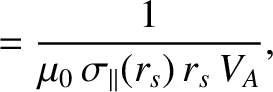
 are the (classical) parallel
electrical conductivity, the ion perpendicular momentum diffusivity, the electron parallel energy diffusivity, the
ion parallel energy diffusivity, the electron perpendicular energy diffusivity, and the ion perpendicular
energy diffusivity, respectively.
are the (classical) parallel
electrical conductivity, the ion perpendicular momentum diffusivity, the electron parallel energy diffusivity, the
ion parallel energy diffusivity, the electron perpendicular energy diffusivity, and the ion perpendicular
energy diffusivity, respectively.


![$\displaystyle = [\phi,\psi] -\left(\frac{\tau}{1+\tau}\right)[N,\psi]
+\hat{\eta}_\parallel\,J + \hat{E}_\parallel,$](img1937.png)

![$\displaystyle = [\phi,N] +c_\beta^{\,2}\,[V,\psi] +\hat{d}_\beta^{\,2}\,[J,\psi] + \hat{\chi}_\parallel\,[[N,\psi],\psi]
+ \hat{\chi}_\perp \hat{\nabla}^{\,2}N,$](img1981.png)

![$\displaystyle = [\phi,U] - \frac{1}{2\,(1+\tau)}\left(\hat{\nabla}^2[\phi,N] + [\hat{\nabla}^2\phi,N] + [\hat{\nabla}^2 N,\phi]\right) + [J,\psi]$](img1982.png)

![$\displaystyle = [\phi,V] +[N,\psi] + \hat{\mit\Xi}_\perp\,\hat{\nabla}^2 V.$](img1983.png)