Next: Perturbed Current Density Up: Toroidal Tearing Modes Previous: Grad-Shafranov Equation Contents
 be the perturbed magnetic field associated with a tearing mode to which the plasma is subject.
Now,
be the perturbed magnetic field associated with a tearing mode to which the plasma is subject.
Now,
 ,
so we obtain
where use has been made of Equation (14.13).
,
so we obtain
where use has been made of Equation (14.13).
It is easily demonstrated from Equations (14.1)–(14.5) that
Suppose, for the moment, that the tearing perturbation has  periods in the poloidal direction and
  periods in the
toroidal direction. Let us adopt the simplifying approximation that the perturbed current density,
periods in the
toroidal direction. Let us adopt the simplifying approximation that the perturbed current density,
 , is negligible in the regions lying between the
various rational surfaces in the plasma [16]. Given that
, is negligible in the regions lying between the
various rational surfaces in the plasma [16]. Given that
 , it follows from Equations (14.13)–(14.15) that
 |
 |
(14.37) |
 |
 |
(14.38) |
 |
 |
(14.39) |
 , the previous three equations imply that
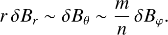 |
(14.40) |
 |
(14.41) |
 smaller than the other two terms. Let us assume that this final term
is negligible, as would be the case in a large aspect-ratio (i.e.,
smaller than the other two terms. Let us assume that this final term
is negligible, as would be the case in a large aspect-ratio (i.e.,
 ) torus. It follows that
where use has been made of Equation (14.3), (14.35), and (14.36). Finally, Equations (14.35) and (14.39) yield
) torus. It follows that
where use has been made of Equation (14.3), (14.35), and (14.36). Finally, Equations (14.35) and (14.39) yield
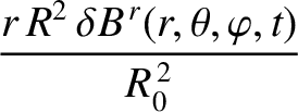
Let
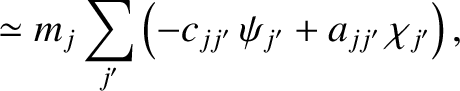
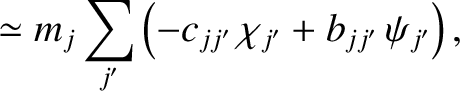
where the sum is over all relevant poloidal harmonics of the perturbed magnetic field. Here, we are now taking account of the fact that a tearing mode in a toroidal tokamak plasma possesses a unique toroidal mode number, but consists of many coupled poloidal harmonics with different poloidal mode numbers [5,6,11,14,22,31]. Operating on Equations (14.42) and (14.43) with , we
obtain
where
, we
obtain
where
 |
 |
(14.48) |
 |
 |
(14.49) |
 |
 |
(14.50) |
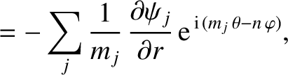
 . This procedure is roughly
equivalent to neglecting the term involving
. This procedure is roughly
equivalent to neglecting the term involving  in the cylindrical tearing mode equation, (3.60). Hence, by analogy
with this equation, we would expect our toroidal tearing mode to be classically stable (given that the
drive for the classical tearing instability in the cylindrical tearing mode equation derives from the term involving ). However, this does not preclude the possibility that our
toroidal tearing mode could be unstable as a neoclassical tearing mode. (See Chapter 12.)
in the cylindrical tearing mode equation, (3.60). Hence, by analogy
with this equation, we would expect our toroidal tearing mode to be classically stable (given that the
drive for the classical tearing instability in the cylindrical tearing mode equation derives from the term involving ). However, this does not preclude the possibility that our
toroidal tearing mode could be unstable as a neoclassical tearing mode. (See Chapter 12.)
Finally, it is readily demonstrated that


![$\displaystyle r\,\frac{\partial}{\partial r}\left(\frac{r\,R^{2}\,\delta B^{\,r...
...}}\right) +\left(\frac{1}{\vert\nabla r\vert^{2}}\right)\delta B_\theta\right],$](img4053.png)
![$\displaystyle r\,\frac{\partial\,\delta B_\theta}{\partial r} \simeq \frac{\par...
...nabla r\cdot\nabla\theta}{\vert\nabla r\vert^{2}}\right)\delta B_\theta\right].$](img4054.png)