Next: Guiding Center Motion Up: Charged Particle Motion Previous: Motion in Uniform Fields Contents
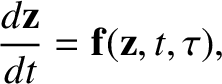
Consider the equation of motion
where is a periodic function of its last argument, with
period
is a periodic function of its last argument, with
period  , and
Here, the small parameter
, and
Here, the small parameter  characterizes the separation between the
short oscillation period and the timescale for the slow secular evolution
of the “position”
characterizes the separation between the
short oscillation period and the timescale for the slow secular evolution
of the “position”  .
.
The basic idea of the averaging method is to treat  and
and  as distinct
independent variables, and to look for solutions of the form
as distinct
independent variables, and to look for solutions of the form
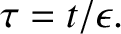
 that are periodic in . Thus, we replace Equation (2.8) by
. All of the secular drifts
are thereby attributed to the variable , while the oscillations are
described entirely by the variable .
Let us denote the -average of by  , and seek a
change of variables of the form
, and seek a
change of variables of the form
   |
(2.11) |
 is a periodic function of with vanishing mean.
Thus,
is a periodic function of with vanishing mean.
Thus,
   |
(2.12) |
 denotes the integral over a full period in .
The evolution of is determined by substituting the
expansions
|
    |
(2.13) |
 |
 |
(2.14) |
.
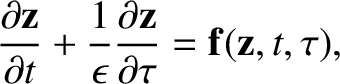
To lowest order, we obtain
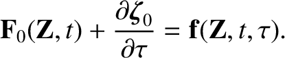
The solubility condition for this equation is Integrating the oscillating component of Equation (2.15) yields![$\displaystyle _0 ({\bf Z}, t,\tau) = \int_0^\tau\left[
{\bf f}({\bf Z},t,\tau') - \langle{\bf f}\rangle({\bf Z},t)\right]d\tau'.$](img262.png) |
(2.17) |
To first order, Equation (2.10) gives,
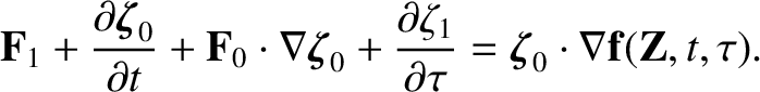 |
(2.18) |
The final result is obtained by combining Equations (2.14), (2.16), and (2.19):
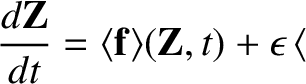  |
(2.20) |
is determined to lowest order by the average of the “force” , and to
next order by the correlation between the oscillation in the “position”
and the
oscillation in the spatial gradient of the “force.”