Next: Method of Averaging Up: Charged Particle Motion Previous: Introduction Contents
 and charge
  in spatially and temporally uniform electromagnetic fields.
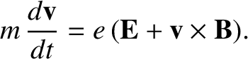
The particle's equation of motion takes the form
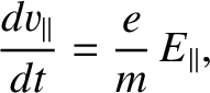
The component of this equation parallel to the magnetic field,
in spatially and temporally uniform electromagnetic fields.
The particle's equation of motion takes the form
The component of this equation parallel to the magnetic field,
 |
(2.2) |
 .
.
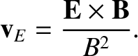
As can easily be verified by substitution, the perpendicular (to the magnetic field) component of Equation (2.1) yields
![$\displaystyle {\bf v}_\perp = \frac{{\bf E}\times{\bf B}}{B^{2}} + \rho\,{\mit\...
... t +\gamma_0) \,{\bf e}_1 +
\cos({\mit\Omega}\, t +\gamma_0)\,{\bf e}_2\right],$](img221.png) |
(2.3) |
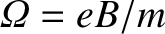 is the gyrofrequency,
  is the gyroradius,
 and
and  are unit vectors such that , ,
  form a
right-handed, mutually orthogonal set, and
form a
right-handed, mutually orthogonal set, and  is the particle's initial
gyrophase. The motion consists of gyration around the
magnetic field at the frequency
is the particle's initial
gyrophase. The motion consists of gyration around the
magnetic field at the frequency
 , superimposed on a
steady drift with velocity
This drift, which is termed the E-cross-B drift,
is identical for all plasma species, and can be eliminated entirely by
transforming to a new inertial frame in which
, superimposed on a
steady drift with velocity
This drift, which is termed the E-cross-B drift,
is identical for all plasma species, and can be eliminated entirely by
transforming to a new inertial frame in which
 .
This frame, which moves with
velocity
.
This frame, which moves with
velocity  with respect to the old frame, can properly be regarded as the rest frame of the plasma.
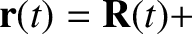
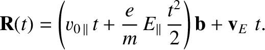
We can complete the previous solution by integrating the velocity to find the particle position. Thus,
   |
(2.5) |
![$\displaystyle (t) = \rho \,[-\cos({\mit\Omega}\, t+\gamma_0)\,{\bf e}_1
+\sin({\mit\Omega}\,t + \gamma_0)\,{\bf e}_2],$](img232.png) |
(2.6) |
 |
(2.7) |
 . Of course, the trajectory of the particle
describes a spiral. The gyrocenter,
. Of course, the trajectory of the particle
describes a spiral. The gyrocenter,  , of this spiral, which is termed
the guiding center, drifts across the magnetic
field with the velocity , and also accelerates along field-lines
at a rate determined by the parallel electric field.
, of this spiral, which is termed
the guiding center, drifts across the magnetic
field with the velocity , and also accelerates along field-lines
at a rate determined by the parallel electric field.
The concept of a guiding center gives us a clue as to how to proceed. Perhaps, when analyzing charged particle motion in nonuniform electromagnetic fields, we can somehow neglect the rapid, and relatively uninteresting, gyromotion, and focus, instead, on the far slower motion of the guiding center? In order to achieve this goal, we need to somehow average the equation of motion over gyrophase, so as to obtain a reduced equation of motion for the guiding center.