Next: Magnetic Energy
Up: Magnetostatics in Magnetic Media
Previous: Soft Iron Sphere in
There are many situations, particularly in experimental physics, where
it is desirable to shield a certain region from magnetic fields. This
goal can be achieved by surrounding the region in question by a material of
high permeability. It is vitally important that a material used as a magnetic
shield does not develop a permanent magnetization in the presence
of external fields, otherwise the material itself
may become a source of magnetic fields. The most effective
commercially available magnetic shielding material is called
mu-metal, and is an alloy of 5 percent copper, 2 percent chromium, 77 percent nickel,
and 16 percent iron. The maximum permeability of mu-metal is about
 .
This material also possesses a particularly low retentivity and coercivity.
Unfortunately, mu-metal is extremely expensive. Let us investigate how
much of this material is actually required to shield a given region
from an external magnetic field.
.
This material also possesses a particularly low retentivity and coercivity.
Unfortunately, mu-metal is extremely expensive. Let us investigate how
much of this material is actually required to shield a given region
from an external magnetic field.
Consider a spherical shell of magnetic shielding, made up of material of
permeability  , placed in a formerly uniform magnetic field
 . Suppose that the inner radius of the
shell is
. Suppose that the inner radius of the
shell is  , and the outer radius is
  . Because there are no free
currents in the problem, we can write
. Because there are no free
currents in the problem, we can write
 .
Furthermore, because
.
Furthermore, because
 and
and
 , it is clear that the magnetic scalar potential satisfies Laplace's
equation,
, it is clear that the magnetic scalar potential satisfies Laplace's
equation,
 , throughout all space. The boundary conditions
are that the potential must be well behaved at
, throughout all space. The boundary conditions
are that the potential must be well behaved at  and
and
 ,
and also that the tangential and the normal components of
,
and also that the tangential and the normal components of  and
and
 , respectively, must be continuous at
  and
and  .
The boundary conditions on
merely imply that the scalar potential
.
The boundary conditions on
merely imply that the scalar potential
 must be continuous at
and
. The boundary
conditions on
yield
must be continuous at
and
. The boundary
conditions on
yield
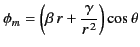
Let us try the following test solution for the magnetic potential:
 |
(745) |
for  ,
,
 |
(746) |
for
 , and
, and
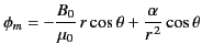
 |
(747) |
for  . This potential is certainly a solution of Laplace's equation
throughout space. It yields the uniform
magnetic field
. This potential is certainly a solution of Laplace's equation
throughout space. It yields the uniform
magnetic field  as
, and satisfies physical boundary conditions at
and infinity.
Because there is a uniqueness theorem associated with Poisson's equation (see Section 2.3),
we can be certain that this potential is the correct solution to the
problem provided that the arbitrary constants
as
, and satisfies physical boundary conditions at
and infinity.
Because there is a uniqueness theorem associated with Poisson's equation (see Section 2.3),
we can be certain that this potential is the correct solution to the
problem provided that the arbitrary constants  ,
,  ,
et cetera, can be adjusted in such a manner that the boundary
conditions at
and
are also satisfied.
,
et cetera, can be adjusted in such a manner that the boundary
conditions at
and
are also satisfied.
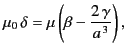
The continuity of
at
and
requires that
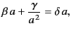 |
(748) |
and
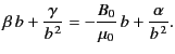 |
(749) |
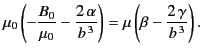
The boundary conditions (744) and (745) yield
 |
(750) |
and
 |
(751) |
It follows that
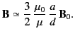
Consider the limit of a thin, high permeability shell for which
 ,
,  , and
, and
 . In this limit, the
field inside the shell is given by
. In this limit, the
field inside the shell is given by
 |
(756) |
Thus, given that
 for mu-metal, we can reduce the magnetic
field-strength inside the shell by almost a factor of 1000 using a shell
whose thickness is only 1/100th of its radius. Note, however, that as the external field-strength,
for mu-metal, we can reduce the magnetic
field-strength inside the shell by almost a factor of 1000 using a shell
whose thickness is only 1/100th of its radius. Note, however, that as the external field-strength,
 , is increased, the mu-metal shell eventually saturates, and
 gradually falls to unity. Thus, extremely strong magnetic
fields (typically,
gradually falls to unity. Thus, extremely strong magnetic
fields (typically,
 tesla) are hardly shielded
at all by mu-metal, or similar magnetic materials.
tesla) are hardly shielded
at all by mu-metal, or similar magnetic materials.
Next: Magnetic Energy
Up: Magnetostatics in Magnetic Media
Previous: Soft Iron Sphere in
Richard Fitzpatrick
2014-06-27
 \,B_0,$](img1566.png)
![$\displaystyle =-\left[ \frac{3\,(2\,\mu+\mu_0)\,\mu_0} {(2\,\mu+\mu_0)\,(\mu+2\,\mu_0) - 2\,(a^{\,3}/b^{\,3})\,(\mu-\mu_0)^{\,2}}\right] B_0,$](img1568.png)
![$\displaystyle = - \left[ \frac{3\,(\mu-\mu_0)\,\mu_0} {(2\,\mu+\mu_0)\,(\mu+2\,\mu_0) - 2\,(a^{\,3}/b^{\,3})\,(\mu-\mu_0)^{\,2}}\right] a^{\,3} B_0,$](img1570.png)
![$\displaystyle = -\left[ \frac{9\,\mu\,\mu_0}{(2\,\mu+\mu_0)\,(\mu+2\,\mu_0) - 2\,(a^{\,3}/b^{\,3})\,(\mu-\mu_0)^{\,2}}\right] B_0.$](img1572.png)