Next: Magnetic Shielding
Up: Magnetostatics in Magnetic Media
Previous: Uniformly Magnetized Sphere
The opposite extreme to a ``hard'' ferromagnetic material, which can maintain
a large remnant magnetization in the absence of external fields, is a
``soft'' ferromagnetic material, for which the remnant magnetization is
relatively small. Let us consider a somewhat idealized situation in which
the remnant magnetization is negligible. In this situation, there is no
hysteresis, so the  -
- relation for the material reduces
to
relation for the material reduces
to
 |
(736) |
where  is a single valued function. The most commonly occurring
``soft'' ferromagnetic material is soft iron (i.e., annealed, low
impurity, iron).
is a single valued function. The most commonly occurring
``soft'' ferromagnetic material is soft iron (i.e., annealed, low
impurity, iron).
Consider a sphere of soft iron placed in an initially uniform external
field
 . The
. The
 and
fields inside the sphere are most easily obtained by taking the solutions (734)
and (735) (which are still valid), and superimposing on them
the uniform field
and
fields inside the sphere are most easily obtained by taking the solutions (734)
and (735) (which are still valid), and superimposing on them
the uniform field  . We are justified in doing this because the
equations that govern magnetostatic problems are linear. Thus, inside
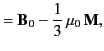
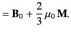
the sphere we have
. We are justified in doing this because the
equations that govern magnetostatic problems are linear. Thus, inside
the sphere we have
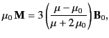
Combining Equations (737), (738), and (739) yields
 |
(739) |
with
 |
(740) |
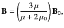
where, in general,
 . Clearly, for a highly permeable material
(i.e.,
. Clearly, for a highly permeable material
(i.e.,
 , which is certainly the case for soft iron) the
magnetic field strength inside the sphere is approximately three times that
of the externally applied field. In other words, the magnetic field
is amplified inside the sphere.
, which is certainly the case for soft iron) the
magnetic field strength inside the sphere is approximately three times that
of the externally applied field. In other words, the magnetic field
is amplified inside the sphere.
The amplification of the magnetic field by a factor three in the high
permeability limit is specific to a sphere. It can be shown that for elongated
objects (e.g., rods), aligned along the direction of the external field,
the amplification factor can be considerably larger than three.
It is important to realize that the magnetization inside a ferromagnetic
material cannot
increase without limit. The maximum possible value of  is
called the saturation magnetization, and is usually denoted
is
called the saturation magnetization, and is usually denoted  .
Most ferromagnetic materials saturate when they are placed in external magnetic
fields whose strengths are greater than, or of order, one tesla. Suppose
that our soft iron sphere first attains the saturation magnetization
when the unperturbed external magnetic field strength is
.
Most ferromagnetic materials saturate when they are placed in external magnetic
fields whose strengths are greater than, or of order, one tesla. Suppose
that our soft iron sphere first attains the saturation magnetization
when the unperturbed external magnetic field strength is  . It follows from
Equations (739) and (740) (with
. It follows from
Equations (739) and (740) (with
 ) that
 |
(741) |
inside the sphere, for  . In this case,
the field amplification factor is
. In this case,
the field amplification factor is
 |
(742) |
Thus, for
 the amplification factor approaches unity. We conclude that
if a ferromagnetic material is placed in an external field that greatly exceeds
that required to cause saturation then the material effectively loses
its magnetic properties, so that
the amplification factor approaches unity. We conclude that
if a ferromagnetic material is placed in an external field that greatly exceeds
that required to cause saturation then the material effectively loses
its magnetic properties, so that
 . Clearly, it is very important
to avoid saturating the soft magnets used to channel magnetic flux around
transformer circuits. This sets an upper limit on the magnetic field-strengths
that can occur in such circuits.
. Clearly, it is very important
to avoid saturating the soft magnets used to channel magnetic flux around
transformer circuits. This sets an upper limit on the magnetic field-strengths
that can occur in such circuits.
Next: Magnetic Shielding
Up: Magnetostatics in Magnetic Media
Previous: Uniformly Magnetized Sphere
Richard Fitzpatrick
2014-06-27