


Next: Dielectric and magnetic media
Up: Electrostatics
Previous: Complex analysis
The method of images and complex analysis are two rather elegant techniques
for solving Poisson's equation. Unfortunately, they both have an
extremely limited range of application. The final technique we shall discuss in this
course, namely, the separation of variables, is somewhat messy,
but possess a far wider range of application. Let us examine a specific
example.
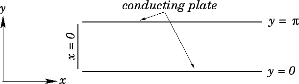
Consider two semi-infinite, grounded, conducting plates lying parallel to the
 -
- plane, one at
  , and the other at
  (see Fig. 46). The left end, at
 , is closed off by an infinite strip insulated from the two plates,
and maintained at a specified potential
, is closed off by an infinite strip insulated from the two plates,
and maintained at a specified potential  . What is the
potential in the region between the plates?
. What is the
potential in the region between the plates?
Figure 46:
 |
We first of all assume that the potential is -independent, since everything else
in the problem is. This reduces the problem to two dimensions.
Poisson's equation is written
 |
(771) |
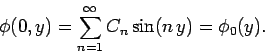
in the vacuum region between the conductors. The boundary conditions are
for  , since the two plates are earthed, plus
 |
(774) |
for
 , and
, and
 |
(775) |
as
 . The latter boundary condition is our usual one for the
scalar potential at infinity.
. The latter boundary condition is our usual one for the
scalar potential at infinity.
The central assumption in the method of separation of variables is that a
multi-dimensional potential can be written as the product of one-dimensional
potentials, so that
 |
(776) |
The above solution is obviously a very special one, and
is, therefore, only likely to satisfy a very small subset of possible
boundary conditions. However, it turns out that by adding together
lots of different solutions of this form we can match to general boundary
conditions.
Substituting (776) into (771), we obtain
 |
(777) |
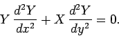
Let us now separate the variables: i.e., let us collect all of the
-dependent terms on one side of the equation, and all of the  -dependent
terms on the other side. Thus,
-dependent
terms on the other side. Thus,
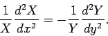 |
(778) |
This equation has the form
 |
(779) |
where  and
and  are general functions. The only way in which the above equation
can be satisfied, for general and , is if both sides are equal to the
same constant. Thus,
are general functions. The only way in which the above equation
can be satisfied, for general and , is if both sides are equal to the
same constant. Thus,
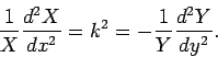 |
(780) |
The reason why we write  , rather than
  , will become apparent later on.
Equation (780) separates into two ordinary differential equations:
, will become apparent later on.
Equation (780) separates into two ordinary differential equations:
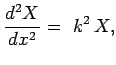 |
|
|
(781) |
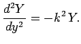 |
|
|
(782) |
We know the general solution to these equations:
giving
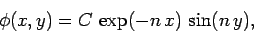
![\begin{displaymath}
\phi = [ A \exp(k x) + B \exp(-k x) ] [C \sin (k y) + D \cos (k y)].
\end{displaymath}](img1620.png) |
(785) |
Here,  ,
,  ,
,  , and
, and  are arbitrary constants. The boundary condition
(775) is automatically satisfied if
are arbitrary constants. The boundary condition
(775) is automatically satisfied if  and
and  .
Note that the choice , instead of
, in Eq. (780) facilitates this by making
.
Note that the choice , instead of
, in Eq. (780) facilitates this by making  either grow or decay
monotonically in the -direction instead of
oscillating. The boundary condition (772)
is automatically
satisfied if
either grow or decay
monotonically in the -direction instead of
oscillating. The boundary condition (772)
is automatically
satisfied if  . The boundary condition (773) is satisfied provided that
 |
(786) |
which implies that  is a positive integer,
  (say). So,
our solution reduces to
(say). So,
our solution reduces to
 |
(787) |
where has been absorbed into . Note that this solution is only able
to satisfy the final boundary condition (774) provided is
proportional to  . Thus, at first sight, it would appear that the method
of separation of variables only works for a very special subset of
boundary conditions. However, this is not the case.
. Thus, at first sight, it would appear that the method
of separation of variables only works for a very special subset of
boundary conditions. However, this is not the case.
Now comes the clever bit! Since Poisson's equation is linear, any
linear combination of solutions is also a solution. We can therefore form a
more general solution than (787) by adding together lots of solutions involving
different values of . Thus,
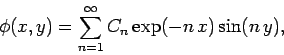 |
(788) |
where the  are constants.
This solution automatically satisfies the boundary conditions (772), (773) and
(775). The
final boundary condition (774) reduces to
are constants.
This solution automatically satisfies the boundary conditions (772), (773) and
(775). The
final boundary condition (774) reduces to
 |
(789) |
The question now is what choice of the fits an arbitrary function
? To answer this question we can make use of two very useful properties
of the functions . Namely, that they are mutually orthogonal, and
form a complete set. The orthogonality property of these functions manifests
itself through the relation
 |
(790) |
where the function
 if
if  and 0 otherwise is called a Kroenecker delta.
The completeness property of sine functions means that any general function
can always be adequately
represented as a weighted sum of sine functions with various different
values. Multiplying both sides of Eq. (789) by
and 0 otherwise is called a Kroenecker delta.
The completeness property of sine functions means that any general function
can always be adequately
represented as a weighted sum of sine functions with various different
values. Multiplying both sides of Eq. (789) by  , and integrating
over , we obtain
, and integrating
over , we obtain
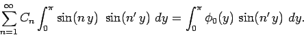 |
(791) |
The orthogonality relation yields
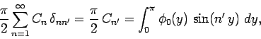 |
(792) |
so
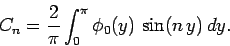 |
(793) |
Thus, we now have a general solution to the problem for any driving potential
.
If the potential is constant then
![\begin{displaymath}
C_n = \frac{2 \phi_0}{\pi} \int_0^\pi \sin (n y) dy
= \frac{2 \phi_0}{n \pi} [1- \cos (n \pi) ],
\end{displaymath}](img1638.png) |
(794) |
giving
 |
(795) |
for even , and
 |
(796) |
for odd . Thus,
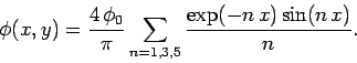 |
(797) |
In the above problem, we write the potential as the product of one-dimensional
functions. Some of these functions grow and decay monotonically (i.e., the
exponential functions), and the others oscillate (i.e., the sinusoidal functions).
The success of the method depends crucially on the orthogonality and completeness
of the oscillatory functions. A set of functions  is orthogonal
if the integral of the product of two different members of the set over some
range is always zero: i.e.,
is orthogonal
if the integral of the product of two different members of the set over some
range is always zero: i.e.,
 |
(798) |
for  . A set of functions is complete if any other function can be
expanded as a weighted sum of them. It turns out that the scheme set out
above can be generalized to more complicated geometries.
For instance, in spherical geometry, the monotonic
functions are power law functions of the radial variable, and the oscillatory functions
are Legendre polynomials. The latter are both mutually orthogonal and form a
complete set. There are also cylindrical, ellipsoidal, hyperbolic, toroidal, etc. coordinates. In all cases, the associated oscillating functions are mutually
orthogonal
and form a complete set. This implies that the method of separation of variables
is of quite general applicability.
. A set of functions is complete if any other function can be
expanded as a weighted sum of them. It turns out that the scheme set out
above can be generalized to more complicated geometries.
For instance, in spherical geometry, the monotonic
functions are power law functions of the radial variable, and the oscillatory functions
are Legendre polynomials. The latter are both mutually orthogonal and form a
complete set. There are also cylindrical, ellipsoidal, hyperbolic, toroidal, etc. coordinates. In all cases, the associated oscillating functions are mutually
orthogonal
and form a complete set. This implies that the method of separation of variables
is of quite general applicability.
Finally, as a simple example of the solution of Poisson's equation in spherical
geometry, let us consider the case of a conducting sphere of radius  , centered on the
origin, placed in a uniform -directed electric field of magnitude
, centered on the
origin, placed in a uniform -directed electric field of magnitude  .
The scalar potential satisfies
.
The scalar potential satisfies
 for
for  , with
the boundary conditions
, with
the boundary conditions
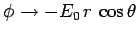 (giving
 ) as
) as
 , and
, and  at
at  . Here,
  and
and  are spherical polar coordinates. Let us try
the simplified separable solution
are spherical polar coordinates. Let us try
the simplified separable solution
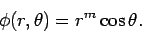 |
(799) |
It is easily demonstrated that the above solution satisfies
provided  or
or  . Thus, the most general solution of
  which satisfies the boundary condition at
is
which satisfies the boundary condition at
is
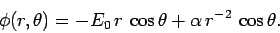 |
(800) |
The boundary condition at is satisfied provided
 |
(801) |
Of course, inside the sphere (i.e.,  ). The charge sheet
density induced on the surface of the sphere is given by
). The charge sheet
density induced on the surface of the sphere is given by
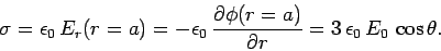 |
(802) |
Next: Dielectric and magnetic media
Up: Electrostatics
Previous: Complex analysis
Richard Fitzpatrick
2006-02-02