Complex analysis

Let us now investigate another trick for solving Poisson's equation (actually it only solves Laplace's equation). Unfortunately, this method can only be applied in two dimensions.

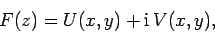
The complex variable is conventionally written

$$z = x + {\rm i} y$$ (740)

($z$ should not be confused with a $z$-coordinate: this is a strictly two-dimensional problem). We can write functions $F(z)$ of the complex variable just like we would write functions of a real variable. For instance,

$$F(z) = z^2,$$ (741)

$$F(z) = \frac{1}{z}.$$ (742)

For a given function, $F(z)$, we can substitute $z=x +{\rm i} y$ and write

$$F(z) = U(x, y) + {\rm i} V(x, y),$$ (743)

where $U$ and $V$ are two real two-dimensional functions. Thus, if

$$F(z) = z^2,$$ (744)

then

$$F(x + {\rm i} y) = (x+{\rm i} y)^2 = (x^2-y^2) + 2 {\rm i} x y,$$ (745)

giving

$$U(x, y) = x^2 - y^2,$$ (746)

$$V(x, y) = 2 x y.$$ (747)

We can define the derivative of a complex function in just the same manner as we would define the derivative of a real function. Thus,

$$\frac{dF}{dz} = _{\lim \vert\delta z\vert\rightarrow\infty} \frac{F(z+\delta z) - F(z) }{\delta z}.$$ (748)

However, we now have a slight problem. If $F(z)$ is a ``well-defined'' function (we shall leave it to the mathematicians to specify exactly what being well-defined entails: suffice to say that most functions we can think of are well-defined) then it should not matter from which direction in the complex plane we approach $z$ when taking the limit in Eq. (748). There are, of course, many different directions we could approach $z$ from, but if we look at a regular complex function, $F(z) = z^2$ (say), then

$$\frac{dF}{dz} = 2 z$$ (749)

is perfectly well-defined, and is, therefore, completely independent of the details of how the limit is taken in Eq. (748).

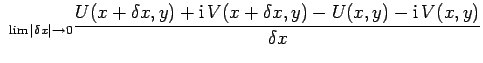
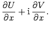
The fact that Eq. (748) has to give the same result, no matter which path we approach $z$ from, means that there are some restrictions on the functions $U$ and $V$ in Eq. (743). Suppose that we approach $z$ along the real axis, so that $\delta z = \delta x$. Then,

$$\frac{dF}{dz} = _{\lim \vert\delta x\vert\rightarrow 0} \frac{U(x+\delta x, y) + {\rm i} V(x+\delta x, y) - U(x, y) - {\rm i} V(x,y)}{\delta x}$$

$$= \frac{\partial U}{\partial x} + {\rm i} \frac{\partial V} {\partial x}.$$ (750)

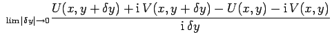
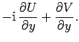
Suppose that we now approach $z$ along the imaginary axis, so that $\delta z = {\rm i} \delta y$. Then,

$$\frac{dF}{dz} = _{\lim \vert\delta y\vert\rightarrow 0} \frac{U(x, y+\delta y) + {\rm i} V(x, y+\delta y) - U(x, y) - {\rm i} V(x,y)}{{\rm i} \delta y}$$

$$= -{\rm i} \frac{\partial U}{\partial y} + \frac{\partial V} {\partial y}.$$ (751)

If $F(z)$ is a well-defined function then its derivative must also be well-defined, which implies that the above two expressions are equivalent. This requires that

$$\frac{\partial U}{\partial x} = \frac{\partial V}{\partial y},$$ (752)

$$\frac{\partial V}{\partial x} = -\frac{\partial U}{\partial y}.$$ (753)

These are called the Cauchy-Riemann relations, and are, in fact, sufficient to ensure that all possible ways of taking the limit (748) give the same answer.

So far, we have found that a general complex function $F(z)$ can be written

$$F(z) = U(x, y) + {\rm i} V(x, y),$$ (754)

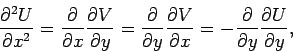
where $z=x +{\rm i} y$. If $F(z)$ is well-defined then $U$ and $V$ automatically satisfy the Cauchy-Riemann relations. But, what has all of this got to do with electrostatics? Well, we can combine the two Cauchy-Riemann relations. We get

$$\frac{\partial^2 U}{\partial x^2} = \frac{\partial}{\partial... ... - \frac{\partial}{\partial y} \frac{\partial U} {\partial y},$$ (755)

and

$$\frac{\partial^2 V}{\partial x^2} = -\frac{\partial}{\partia... ... - \frac{\partial}{\partial y} \frac{\partial V} {\partial y},$$ (756)

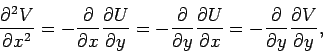
which reduce to

$$\frac{\partial^2 U}{\partial x^2} + \frac{\partial^2 U}{\partial y^2} = 0,$$ (757)

$$\frac{\partial^2 V}{\partial x^2} + \frac{\partial^2 V}{\partial y^2} = 0.$$ (758)

Thus, both $U$ and $V$ automatically satisfy Laplace's equation in two dimensions; i.e., both $U$ and $V$ are possible two-dimensional scalar potentials in free space.

Consider the two-dimensional gradients of $U$ and $V$:

$$\nabla U = \left( \frac{\partial U}{\partial x}, \frac{\partial U}{\partial y} \right),$$ (759)

$$\nabla V = \left( \frac{\partial V}{\partial x}, \frac{\partial V}{\partial y} \right).$$ (760)

Now

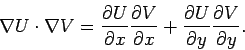$$\nabla U \cdot \nabla V = \frac{\partial U}{\partial x}\frac... ... +\frac{\partial U}{\partial y} \frac{\partial V}{\partial y}.$$ (761)

It follows from the Cauchy-Riemann relations that

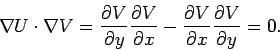$$\nabla U \cdot \nabla V = \frac{\partial V}{\partial y}\frac... ...\frac{\partial V}{\partial x} \frac{\partial V}{\partial y}=0.$$ (762)

Thus, the contours of $U$ are everywhere perpendicular to the contours of $V$. It follows that if $U$ maps out the contours of some free space scalar potential then $V$ indicates the directions of the associated electric field-lines, and vice versa.

Figure 45:

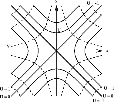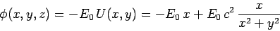
For every well-defined complex function we can think of, we get two sets of free space potentials, and the associated electric field-lines. For example, consider the function $F(z) = z^2$, for which

$$U = x^2 - y^2,$$ (763)

$$V = 2 x y.$$ (764)

These are, in fact, the equations of two sets of orthogonal hyperboloids. So, $U(x,y)$ (the solid lines in Fig. 45) might represent the contours of some scalar potential and $V(x,y)$ (the dashed lines in Fig. 45) the associated electric field lines, or vice versa. But, how could we actually generate a hyperboloidal potential? This is easy. Consider the contours of $U$ at level $\pm 1$. These could represent the surfaces of four hyperboloid conductors maintained at potentials $\pm \cal V$. The scalar potential in the region between these conductors is given by ${\cal V} U(x, y)$, and the associated electric field-lines follow the contours of $V(x,y)$. Note that

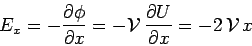$$E_x = - \frac{\partial\phi}{\partial x} =- {\cal V} \frac{\partial U}{\partial x} = -2 {\cal V} x$$ (765)

Thus, the $x$-component of the electric field is directly proportional to the distance from the $x$-axis. Likewise, for $y$-component of the field is directly proportional to the distance from the $y$-axis. This property can be exploited to make devices (called quadrupole electrostatic lenses) which are useful for focusing particle beams.

As a second example, consider the complex function

$$F(z) = z - \frac{c^2}{z},$$ (766)

where $c$ is real and positive. Writing $F(z)=U(x,y) + {\rm i} V(x,y)$, we find that

$$U(x,y) = x - \frac{c^2 x}{x^2+y^2}.$$ (767)

Far from the origin, $U\rightarrow x$, which is the potential of a uniform electric field, of unit amplitude, pointing in the $-x$-direction. The locus of $U=0$ is $x=0$, and

$$x^2+y^2 = c^2,$$ (768)

which corresponds to a circle of radius $c$ centered on the origin. Hence, we conclude that the potential

$$\phi(x,y,z) = - E_0 U(x,y) = -E_0 x + E_0 c^2 \frac{x}{x^2+y^2}$$ (769)

corresponds to that outside a grounded, infinitely long, conducting cylinder of radius $c$, running parallel to the $z$-axis, placed in a uniform $x$-directed electric field of magnitude $E_0$. Of course, the potential inside the cylinder (i.e., $x^2+y^2< c^2$) is zero. The induced charge density on the surface of the cylinder is simply

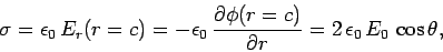$$\sigma = \epsilon_0 E_r(r=c) = - \epsilon_0 \frac{\partial\phi(r=c)}{\partial r} = 2 \epsilon_0 E_0 \cos\theta,$$ (770)

where $r^2 = x^2+y^2$, and $x= r \cos\theta$. Note that zero net charge is induced on the surface.

We can think of the set of all possible well-defined complex functions as a reference library of solutions to Laplace's equation in two dimensions. We have only considered a couple of examples, but there are, of course, very many complex functions which generate interesting potentials. For instance, $F(z) = z^{1/2}$ generates the potential around a semi-infinite, thin, grounded, conducting plate placed in an external field, whereas $F(z) = z^{3/2}$ yields the potential outside a grounded, rectangular, conducting corner under similar circumstances.