| (257) |
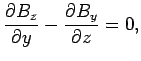
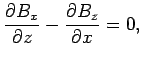
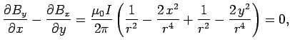
Let us evaluate
![]() directly. According to Eq. (254),
directly. According to Eq. (254),
| (265) |
But, why have we gone to so much trouble to prove
something using vector field theory which can be demonstrated
in one line via conventional
analysis [see Eq. (258)]? The answer, of course, is that the vector field
result is easily generalized, whereas the
conventional result is just a special case.
For instance, it is clear that Eq. (266) is true for any surface attached to the loop
C, not just a plane surface.
Moreover, suppose that we distort our simple circular loop ![]() so that it is no longer circular or even lies in one plane.
What now is the line integral
of
so that it is no longer circular or even lies in one plane.
What now is the line integral
of ![]() around the loop? This is no longer a simple problem for conventional
analysis, because the magnetic field is not parallel to a line element of the
loop.
However, according to Stokes' theorem,
around the loop? This is no longer a simple problem for conventional
analysis, because the magnetic field is not parallel to a line element of the
loop.
However, according to Stokes' theorem,
| (267) |
| (268) |
Thus, provided the curve ![]() circulates the
circulates the ![]() -axis, and, therefore, any surface
-axis, and, therefore, any surface
![]() attached to
attached to ![]() intersects the
intersects the ![]() -axis, the line integral
-axis, the line integral
![]() is equal to
is equal to ![]() .
Of course, if
.
Of course, if ![]() does not circulate the
does not circulate the ![]() -axis then
an attached surface
-axis then
an attached surface ![]() does not intersect the
does not intersect the ![]() -axis and
-axis and
![]() is zero. There is one more proviso. The line
integral
is zero. There is one more proviso. The line
integral
![]() is
is ![]() for a loop which circulates the
for a loop which circulates the
![]() -axis in a clockwise direction (looking up the
-axis in a clockwise direction (looking up the
![]() -axis). However, if the loop circulates in an anti-clockwise
direction then the integral is
-axis). However, if the loop circulates in an anti-clockwise
direction then the integral is ![]() . This follows because in the latter case
the
. This follows because in the latter case
the ![]() -component of the surface element
-component of the surface element ![]() is oppositely directed to
the current flow at the point where the surface intersects the wire.
is oppositely directed to
the current flow at the point where the surface intersects the wire.
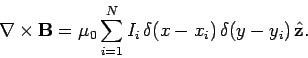
Let us now consider ![]() wires directed along the
wires directed along the ![]() -axis, with coordinates
(
-axis, with coordinates
(![]() ,
, ![]() ) in the
) in the ![]() -
-![]() plane, each carrying a current
plane, each carrying a current ![]() in the
positive
in the
positive ![]() -direction. It is fairly obvious that Eq. (264) generalizes
to
-direction. It is fairly obvious that Eq. (264) generalizes
to
Equation (269) is a field equation describing how a set of ![]() -directed
current carrying wires generate a magnetic field. These wires have
zero-thickness, which implies that we are trying to squeeze a finite amount of
current into an infinitesimal region. This
accounts for the delta-functions on the right-hand side of
the equation. Likewise, we obtained delta-functions in Sect. 3.4
because we were dealing with point charges. Let us now generalize to the more
realistic case of diffuse currents. Suppose that the
-directed
current carrying wires generate a magnetic field. These wires have
zero-thickness, which implies that we are trying to squeeze a finite amount of
current into an infinitesimal region. This
accounts for the delta-functions on the right-hand side of
the equation. Likewise, we obtained delta-functions in Sect. 3.4
because we were dealing with point charges. Let us now generalize to the more
realistic case of diffuse currents. Suppose that the ![]() -current flowing through
a small
rectangle in the
-current flowing through
a small
rectangle in the ![]() -
-![]() plane, centred on coordinates (
plane, centred on coordinates (![]() ,
, ![]() ) and of dimensions
) and of dimensions
![]() and
and ![]() , is
, is
![]() . Here,
. Here, ![]() is termed the current density in
the
is termed the current density in
the ![]() -direction. Let us integrate
-direction. Let us integrate
![]() over this rectangle.
The rectangle is assumed to be sufficiently small that
over this rectangle.
The rectangle is assumed to be sufficiently small that
![]() does not vary appreciably across it. According to Eq. (270), this integral is
equal to
does not vary appreciably across it. According to Eq. (270), this integral is
equal to ![]() times the total
times the total ![]() -current flowing through the rectangle. Thus,
-current flowing through the rectangle. Thus,
| (271) |
| (273) |
If we form the line integral of ![]() around some general closed curve
around some general closed curve
![]() , making use of Stokes' theorem and the field equation (274), then we
obtain
, making use of Stokes' theorem and the field equation (274), then we
obtain
The flux of the current density
through ![]() is evaluated by integrating
is evaluated by integrating
![]() over any surface
over any surface
![]() attached to
attached to ![]() . Suppose that we take two different surfaces
. Suppose that we take two different surfaces ![]() and
and
![]() . It is clear that if Ampère's circuital
law is to make any sense then the surface integral
. It is clear that if Ampère's circuital
law is to make any sense then the surface integral
![]() had better equal the integral
had better equal the integral
![]() . That is, when we work out the flux of the current
though
. That is, when we work out the flux of the current
though ![]() using two different attached surfaces then we had better get
the same answer, otherwise Eq. (275) is wrong (since the left-hand side is clearly independent
of the surface spanning C).
We saw in Sect. 2 that if the integral of a vector field
using two different attached surfaces then we had better get
the same answer, otherwise Eq. (275) is wrong (since the left-hand side is clearly independent
of the surface spanning C).
We saw in Sect. 2 that if the integral of a vector field ![]() over some surface attached to a loop depends only on the loop, and is
independent of the surface which spans it, then this implies that
over some surface attached to a loop depends only on the loop, and is
independent of the surface which spans it, then this implies that
![]() . The flux of the current
density through any loop
. The flux of the current
density through any loop ![]() is calculated by evaluating the integral
is calculated by evaluating the integral
![]() for
any surface
for
any surface ![]() which spans the loop. According to
Ampère's circuital law, this integral depends only on
which spans the loop. According to
Ampère's circuital law, this integral depends only on ![]() and is completely independent of
and is completely independent of ![]() (i.e., it is equal to the line integral of
(i.e., it is equal to the line integral of ![]() around
around ![]() , which depends
on
, which depends
on ![]() but not on
but not on ![]() ). This implies that
). This implies that
![]() . In fact, we
can obtain this relation directly from the field equation (274). We know that
the divergence of a curl is automatically zero, so taking the divergence
of Eq. (274), we obtain
. In fact, we
can obtain this relation directly from the field equation (274). We know that
the divergence of a curl is automatically zero, so taking the divergence
of Eq. (274), we obtain
| (276) |
We have shown that if Ampère's circuital law is to make any sense then we need
![]() . Physically, this implies that the net current flowing
through any closed surface
. Physically, this implies that the net current flowing
through any closed surface ![]() is zero.
Up to now, we have only considered
stationary charges and steady currents. It is clear that if all charges are
stationary and all currents are steady then there can be no net current flowing
through a closed surface
is zero.
Up to now, we have only considered
stationary charges and steady currents. It is clear that if all charges are
stationary and all currents are steady then there can be no net current flowing
through a closed surface ![]() , since this would imply a build up of charge in the
volume
, since this would imply a build up of charge in the
volume ![]() enclosed by
enclosed by ![]() . In other words, as long as we restrict our investigation
to stationary charges, and steady currents, then we expect
. In other words, as long as we restrict our investigation
to stationary charges, and steady currents, then we expect
![]() ,
and Ampère's circuital law makes sense. However, suppose that we now relax this
restriction. Suppose that some of the charges in a volume
,
and Ampère's circuital law makes sense. However, suppose that we now relax this
restriction. Suppose that some of the charges in a volume ![]() decide to move
outside
decide to move
outside ![]() . Clearly, there will be a non-zero net flux of electric current through
the bounding surface
. Clearly, there will be a non-zero net flux of electric current through
the bounding surface ![]() whilst this is happening. This implies from
Gauss' theorem that
whilst this is happening. This implies from
Gauss' theorem that
![]() . Under these circumstances
Ampère's circuital law collapses in a heap. We shall see later that we can rescue
Ampère's circuital law by adding an extra term involving a time derivative to the
right-hand side of the field equation (274).
For steady-state situations (i.e.,
. Under these circumstances
Ampère's circuital law collapses in a heap. We shall see later that we can rescue
Ampère's circuital law by adding an extra term involving a time derivative to the
right-hand side of the field equation (274).
For steady-state situations (i.e.,
![]() ), this
extra term can be neglected. Thus, the field equation
), this
extra term can be neglected. Thus, the field equation
![]() is, in fact, only two-thirds of Maxwell's third equation: there is a term missing
on the right-hand side.
is, in fact, only two-thirds of Maxwell's third equation: there is a term missing
on the right-hand side.
We have now derived two field equations involving magnetic fields (actually,
we have only derived one
and two-thirds):