![[*]](footnote.png) Furthermore, let us investigate any changes which
may develop in the nature of the
pendulum's time-asymptotic motion
as the quality-factor
Furthermore, let us investigate any changes which
may develop in the nature of the
pendulum's time-asymptotic motion
as the quality-factor
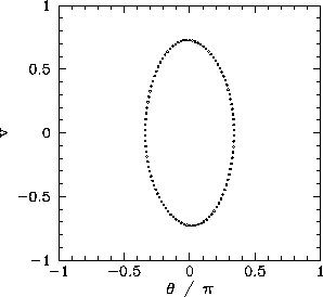 |
Figure 62 shows a time-asymptotic orbit in phase-space
calculated numerically for a case where ![]() is sufficiently
small (i.e.,
is sufficiently
small (i.e., ![]() ) that the small angle approximation holds reasonably well. Not surprisingly,
the orbit is very similar to the analytic orbits
described in Section 15.3. The fact that the orbit consists
of a single loop, and forms a closed curve in phase-space,
strongly suggests that the corresponding
motion is periodic with the same period as the external drive--we term this type of motion
period-1 motion. More generally, period-
) that the small angle approximation holds reasonably well. Not surprisingly,
the orbit is very similar to the analytic orbits
described in Section 15.3. The fact that the orbit consists
of a single loop, and forms a closed curve in phase-space,
strongly suggests that the corresponding
motion is periodic with the same period as the external drive--we term this type of motion
period-1 motion. More generally, period-![]() motion consists of motion which
repeats itself exactly every
motion consists of motion which
repeats itself exactly every ![]() periods of the external drive (and, obviously,
does not repeat itself on any time-scale less than
periods of the external drive (and, obviously,
does not repeat itself on any time-scale less than ![]() periods). Of course, period-1 motion
is the only allowed time-asymptotic motion in the small angle limit.
periods). Of course, period-1 motion
is the only allowed time-asymptotic motion in the small angle limit.
It would certainly be helpful
to possess a graphical test for period-![]() motion. In fact, such a test was developed more than a
hundred years ago by the
French mathematician Henry Poincaré. Nowadays, it is called a
Poincaré section in his honour. The idea of a Poincaré section, as applied
to a periodically driven pendulum, is very simple.
As before, we calculate the time-asymptotic motion of the pendulum, and visualize it as a
series of points in
motion. In fact, such a test was developed more than a
hundred years ago by the
French mathematician Henry Poincaré. Nowadays, it is called a
Poincaré section in his honour. The idea of a Poincaré section, as applied
to a periodically driven pendulum, is very simple.
As before, we calculate the time-asymptotic motion of the pendulum, and visualize it as a
series of points in ![]() -
-![]() phase-space. However, we only plot one point per period of the external drive. To be more
exact, we only plot a point when
phase-space. However, we only plot one point per period of the external drive. To be more
exact, we only plot a point when
| (1250) |
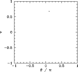 |
Figure 63 displays the Poincaré section of the orbit shown in Figure 62. The fact that the section consists of a single point confirms that the motion displayed in Figure 62 is indeed period-1 motion.