| (1239) |
The linearized equations of motion of the pendulum take the form:
 |
(1244) |
 |
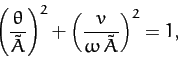
It is often convenient to visualize the motion of a dynamical system as an orbit, or trajectory, in
phase-space, which is defined as the space of all of the dynamical variables required to
specify the instantaneous state of the system. For the case in hand, there are two dynamical
variables, ![]() and
and ![]() , and so phase-space corresponds to the
, and so phase-space corresponds to the ![]() -
-![]() plane. Note that
each different point in this plane corresponds to a unique instantaneous state of the pendulum.
[Strictly speaking, we should also consider
plane. Note that
each different point in this plane corresponds to a unique instantaneous state of the pendulum.
[Strictly speaking, we should also consider ![]() to be a dynamical variable, since it
appears explicitly on the right-hand side of Equation (1238).]
to be a dynamical variable, since it
appears explicitly on the right-hand side of Equation (1238).]
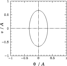
It is clear, from Equations (1242) and (1243), that if we wait long enough for all
of the transients to decay away then the motion of the pendulum settles down to the
following simple orbit in phase-space:
![$\displaystyle \frac{A\left[(1-\omega^2)\,\cos(\omega\, t)+ (\omega/Q)\,\sin(\omega\, t)\right]}
{\left[(1-\omega^2)^2+\omega^2/Q^2\right]},$](img3055.png) |
(1245) | ||
![$\displaystyle \frac{\omega\, A\left[-(1-\omega^2)\,\sin(\omega\, t)+ (\omega/Q)\,\cos(\omega\, t)\right]}
{\left[(1-\omega^2)^2+\omega^2/Q^2\right]}.$](img3056.png) |
(1246) |
 |
(1247) |
| (1249) |
 |
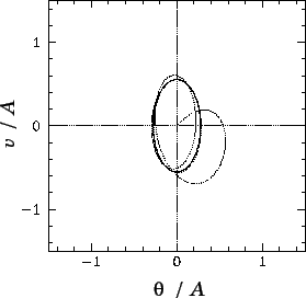
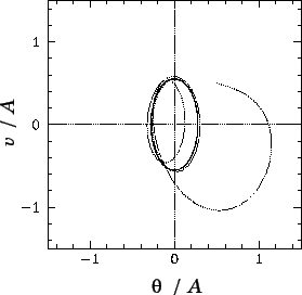
The phase-space curve shown in Figure 58 is called a periodic attractor. It is
termed an ``attractor'' because,
irrespective of the initial conditions, the trajectory of the system in phase-space tends
asymptotically to--in other words, is attracted to--this curve as
![]() . This
gravitation of phase-space trajectories towards the attractor is illustrated in Figures 60 and
61. Of course, the attractor is termed ``periodic'' because it corresponds to motion which is
periodic in time.
. This
gravitation of phase-space trajectories towards the attractor is illustrated in Figures 60 and
61. Of course, the attractor is termed ``periodic'' because it corresponds to motion which is
periodic in time.
 |
 |
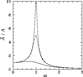
Let us summarize our findings so far. We have discovered that if a damped pendulum is subject to a low amplitude periodic drive then its time-asymptotic response (i.e., its response after any transients have died away) is periodic, with the same period as the driving torque. Moreover, the response exhibits resonant behaviour as the driving frequency approaches the natural frequency of oscillation of the pendulum. The amplitude of the resonant response, as well as the width of the resonant window, is governed by the amount of damping in the system. After a little reflection, we can easily appreciate that all of these results are a direct consequence of the linearity of the pendulum's equations of motion in the low amplitude limit. In fact, it is easily demonstrated that the time-asymptotic response of any intrinsically stable linear system (with a discrete spectrum of normal modes) to a periodic drive is periodic, with the same period as the drive. Moreover, if the driving frequency approaches one of the natural frequencies of oscillation of the system then the response exhibits resonant behaviour. But, is this the only allowable time-asymptotic response of a dynamical system to a periodic drive? It turns out that it is not. Indeed, the response of a non-linear system to a periodic drive is generally much richer and far more diverse than simple periodic motion. Since the majority of naturally occurring dynamical systems are non-linear, it is clearly important that we gain a basic understanding of this phenomenon. Unfortunately, we cannot achieve this goal via a standard analytic approach, since non-linear equations of motion generally do not possess simple analytic solutions. Instead, we must employ numerical methods. As an example, let us investigate the dynamics of a damped pendulum, subject to a periodic drive, with no restrictions on the amplitude of the pendulum's motion.
![$\displaystyle \left\{\theta(0) - \frac{A\,(1-\omega^2)}{[(1-\omega^2)^2+\omega^2/Q^2]}\right\}
{\rm e}^{-t/2Q}\,\cos(\omega_\ast\, t)$](img3044.png)
![$\displaystyle +\frac{1}{\omega_\ast}\left\{ v(0) + \frac{\theta(0)}{2Q}
-\frac{...
...}
{[(1-\omega^2)^2+ \omega^2/Q^2]}\right\}{\rm e}^{-t/2Q}\,\sin(\omega_\ast\,t)$](img3045.png)
![$\displaystyle +\frac{A\left[(1-\omega^2)\,\cos(\omega\, t)+ (\omega/Q)\,\sin(\omega\, t)\right]}
{\left[(1-\omega^2)^2+\omega^2/Q^2\right]},$](img3046.png)
![$\displaystyle \left\{v(0) - \frac{A\,\omega^2/Q}{[(1-\omega^2)^2+\omega^2/Q^2]}\right\}
{\rm e}^{-t/2Q}\,\cos\omega_\ast t$](img3048.png)
![$\displaystyle -\frac{1}{\omega_\ast}\left\{ \theta(0) + \frac{v(0)}{2Q}
-\frac{...
...
{[(1-\omega^2)^2+ \omega^2/Q^2]}\right\}{\rm e}^{-t/2Q}\,\sin(\omega_\ast\, t)$](img3049.png)
![$\displaystyle +\frac{\omega\,A\left[-(1-\omega^2)\,\sin(\omega\, t)+ (\omega/Q)\,\cos(\omega\, t)\right]}
{\left[(1-\omega^2)^2+\omega^2/Q^2\right]}.$](img3050.png)