Axisymmetric Velocity Fields

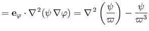
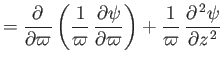
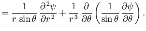
According to the analysis of Appendix C, Equations (7.3) and (7.4) imply that

$${\bf v} = \nabla\varphi\times \nabla \psi.$$ (7.5)

When the fluid velocity is written in this form it becomes obvious that the incompressibility constraint $\nabla\cdot{\bf v}=0$ is satisfied [because $\nabla\cdot(\nabla A\times \nabla B)\equiv 0$ --see Equations (A.175) and (A.176)]. It is also clear that the Stokes stream function, $\psi$ , is undefined to an arbitrary additive constant.

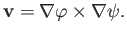
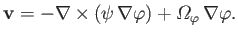
In fact, the most general expression for an axisymmetric incompressible flow pattern is

$${\bf v} = \nabla\varphi\times\nabla\psi + {\mit\Omega}_\varphi\,\nabla\varphi,$$ (7.6)

where ${\mit\Omega}_\varphi={\mit\Omega}_\varphi(\varpi,z)$ is the angular velocity of flow circulating about the $z$ -axis. (This follows because $\nabla\cdot ({\mit\Omega}_\varphi\,\nabla\varphi)=0$ when $\partial{\mit\Omega}_\varphi/\partial\varphi=0$ . See Appendix C.) The previous expression implies that ${\bf v}\cdot\nabla\psi = 0$ (because $\nabla\psi\cdot\nabla\varphi=0$ when $\partial\psi/\partial\varphi=0$ ). In other words, when plotted in the meridian plane, streamlines in a general axisymmetric flow pattern correspond to contours of $\psi$ .

Making use of the vector identities (A.176) and (A.178), we can also write Equation (7.6) in the form

$${\bf v} = -\nabla\times (\psi\,\nabla\varphi) + {\mit\Omega}_\varphi\,\nabla\varphi.$$ (7.7)

It follows from the identity (A.177) that

$$\nabla\times {\bf v} = -\nabla[\nabla\cdot(\psi\,\nabla\varphi)] + \nabla^{\,2}(\psi\,\nabla\varphi)+\nabla{\mit\Omega}_\varphi\times \nabla\varphi$$

$$= \nabla^{\,2}(\psi\,\nabla\varphi)+\nabla{\mit\Omega}_\varphi\times \nabla\varphi,$$ (7.8)

because $\nabla\cdot(\psi\,\nabla\varphi)=0$ , by symmetry. Hence, the vorticity of a general axisymmetric flow pattern is written

$$\mbox{\boldmath$\omega$} = \nabla{\mit\Omega}_\varphi\times \nabla\varphi + \omega_\varphi\,{\bf e}_\varphi,$$ (7.9)

where $\omega_\varphi=\omega_\varphi(\varpi,z)$ , and [see Equations (C.52)-(C.54)]

$$\omega_\varphi = {\bf e}_\varphi\cdot\nabla^{\,2}(\psi\,\nabla\varphi)= \nabla^{\,2}\left(\frac{\psi}{\varpi}\right)-\frac{\psi}{\varpi^3}$$

$$=\frac{\partial}{\partial\varpi}\left(\frac{1}{\varpi}\,\frac{\pa... ...l\varpi}\right) + \frac{1}{\varpi}\,\frac{\partial^{\,2}\psi}{\partial z^{\,2}}$$

$$= \frac{1}{r\,\sin\theta}\,\frac{\partial^{\,2}\psi}{\partial r^{... ...\theta}\left( \frac{1}{\sin\theta}\,\frac{\partial\psi}{\partial\theta}\right).$$ (7.10)

In the following, we shall concentrate on axisymmetric flow patterns in which there is no circulation about the $z$ -axis (i.e., ${\mit\Omega}_\varphi=v_\varphi=0$ ).