


Next: Jacobi Ellipsoids
Up: Hydrostatics
Previous: Equilibrium of a Rotating
One, fairly obvious, way in which the constraint (2.115) can be satisfied is if  . In other words, if the planet is rotationally symmetric about its axis of rotation. An ellipsoid that is rotationally symmetric about a
principal axis--or, equivalently, an ellipsoid with two equal principal radii--is known as a spheroid.
In fact, if
then the cross-section of the planet's outer boundary in any plane passing though the
. In other words, if the planet is rotationally symmetric about its axis of rotation. An ellipsoid that is rotationally symmetric about a
principal axis--or, equivalently, an ellipsoid with two equal principal radii--is known as a spheroid.
In fact, if
then the cross-section of the planet's outer boundary in any plane passing though the  -axis is
an ellipse of major radius
-axis is
an ellipse of major radius  in the direction perpendicular to the
-axis, and minor radius
in the direction perpendicular to the
-axis, and minor radius  in the direction parallel to the
-axis. Here, we are assuming that
in the direction parallel to the
-axis. Here, we are assuming that  : that is, the
planet is flattened along its axis of rotation. The degree of flattening is conveniently
measured by the eccentricity,
: that is, the
planet is flattened along its axis of rotation. The degree of flattening is conveniently
measured by the eccentricity,
 |
(2.118) |
Thus, if  then there is no flattening, and the planet is consequently spherical, whereas if
 then the flattening is complete, and the planet consequently collapses to a disk in the
  -
- plane.
Let
 and
and
 . Setting
in Equation (2.114), we obtain
. Setting
in Equation (2.114), we obtain
Performing the integrals, which are standard (Speigel, Liu, and Lipschutz 1999),
we find that
 |
(2.120) |
This famous result was first obtained by Colin Maclaurin (1698-1746) in 1742.
Finally, in order to calculate the potential energy, (2.116), we need to evaluate
Table 2.1:
Properties of the Maclaurin spheroids.
| |
|
|
|
|
|
|
|

|

|

|

|
|
|
|
|
| |
|
|
|
|
|
|
|
| 0.00 |
0.00000 |
0.00000 |
0.60000 |
0.60 |
0.31729 |
0.18037 |
0.56233 |
| 0.05 |
0.02582 |
0.01266 |
0.59980 |
0.65 |
0.34484 |
0.20286 |
0.55320 |
| 0.10 |
0.05168 |
0.02540 |
0.59919 |
0.70 |
0.37239 |
0.22834 |
0.54200 |
| 0.15 |
0.07758 |
0.03830 |
0.59817 |
0.75 |
0.39967 |
0.25792 |
0.52800 |
| 0.20 |
0.10357 |
0.05144 |
0.59672 |
0.80 |
0.42612 |
0.29345 |
0.51001 |
| 0.25 |
0.12967 |
0.06491 |
0.59479 |
0.85 |
0.45046 |
0.33833 |
0.48587 |
| 0.30 |
0.15591 |
0.07882 |
0.59236 |
0.90 |
0.46932 |
0.39994 |
0.45107 |
| 0.35 |
0.18231 |
0.09329 |
0.58936 |
0.95 |
0.47045 |
0.50074 |
0.39272 |
| 0.40 |
0.20889 |
0.10846 |
0.58572 |
0.96 |
0.46472 |
0.53194 |
0.37485 |
| 0.45 |
0.23567 |
0.12450 |
0.58135 |
0.97 |
0.45418 |
0.57123 |
0.35273 |
| 0.50 |
0.26267 |
0.14163 |
0.57612 |
0.98 |
0.43475 |
0.62486 |
0.32351 |
| 0.55 |
0.28989 |
0.16013 |
0.56986 |
0.99 |
0.39389 |
0.71209 |
0.27916 |
|
Let
 . Thus,
  corresponds to no rotational flattening, and
 to complete flattening.
Moreover,
to complete flattening.
Moreover,
 and
and
 , where
 is the mean radius.
It is also helpful to define
is the mean radius.
It is also helpful to define
 ,
,
 , and
, and
 . The previous analysis leads to
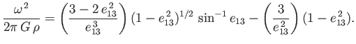
the following set of equations that specify the properties of the so-called Maclaurin spheroids:
. The previous analysis leads to
the following set of equations that specify the properties of the so-called Maclaurin spheroids:
These properties are set out
in Table 2.1.
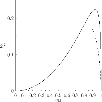
Figure:
Normalized angular velocity squared of a Maclaurin spheroid (solid) and a Jacobi
ellipsoid (dashed) versus the eccentricity
in the
-
plane.
 |
In the limit,
 , in which the planet is relatively
slowly rotating (i.e.,
, in which the planet is relatively
slowly rotating (i.e.,
 ), and its degree of flattening consequently slight, Equations (2.122)-(2.124) reduce to
In other words, in the limit of relatively slow rotation, when the planet is almost spherical, its eccentricity
becomes directly proportional to its angular velocity. In this case, it is more conventional to parameterize angular velocity in terms of
 |
(2.128) |
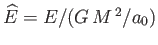
where
 is the mean surface gravitational acceleration.
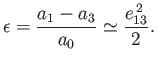
Furthermore, the degree of rotational flattening is more conveniently expressed in terms of the ellipticity,
is the mean surface gravitational acceleration.
Furthermore, the degree of rotational flattening is more conveniently expressed in terms of the ellipticity,
 |
(2.129) |
Thus, it follows from (2.125) that
 |
(2.130) |
For the case of the Earth (
 ,
,
 ,
,
 --Yoder 1995), we obtain
 |
(2.131) |
Thus, it follows that, were the Earth homogeneous, its figure would be a spheroid, flattened at the poles, of ellipticity
 |
(2.132) |
This result was first obtained by Newton.
The actual ellipticity of the Earth is about  (Yoder 1995), which is substantially smaller than Newton's prediction. The
discrepancy is due to the fact that the Earth is strongly inhomogeneous, being much denser at its core than in its
outer regions.
(Yoder 1995), which is substantially smaller than Newton's prediction. The
discrepancy is due to the fact that the Earth is strongly inhomogeneous, being much denser at its core than in its
outer regions.
Figure:
Normalized angular momentum of a Maclaurin spheroid (solid) and a Jacobi
ellipsoid (dashed) versus the eccentricity
in the
-
plane.
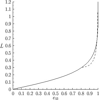 |
Figures 2.5 and 2.6 illustrate the variation of the normalized angular velocity,
, and angular
momentum,
, of a Maclaurin spheroid with its eccentricity,
, as predicted by Equations (2.122)-(2.124).
It can be seen, from Figure 2.5, that there is a limit to how large the normalized angular velocity of such a spheroid
can become. The limiting value corresponds to
 , and
occurs when
, and
occurs when
 . For values of
lying below
. For values of
lying below  there are
two possible Maclaurin spheroids, one with an eccentricity less than
there are
two possible Maclaurin spheroids, one with an eccentricity less than  , and one with an
eccentricity greater than
. Note, however, from Figure 2.6, that despite the fact that the
angular velocity,
, of a Maclaurin spheroid varies in a non-monotonic manner with the eccentricity,
, the
angular momentum,
, increases monotonically with
, becoming infinite in the
limit
. It follows that there
is no upper limit to the angular momentum of a Maclaurin spheroid.
, and one with an
eccentricity greater than
. Note, however, from Figure 2.6, that despite the fact that the
angular velocity,
, of a Maclaurin spheroid varies in a non-monotonic manner with the eccentricity,
, the
angular momentum,
, increases monotonically with
, becoming infinite in the
limit
. It follows that there
is no upper limit to the angular momentum of a Maclaurin spheroid.
Next: Jacobi Ellipsoids
Up: Hydrostatics
Previous: Equilibrium of a Rotating
Richard Fitzpatrick
2016-03-31

![$\displaystyle = \frac{2\,(1-e_{13}^{\,2})^{1/2}}{e_{13}^{\,3}}\left[\int_0^{e_{...
...}}-(1-e_{13}^{\,2})\int_0^{e_{13}}\frac{z^{\,2}\,dz}{(1-z^{\,2})^{3/2}}\right].$](img880.png)


![$\displaystyle =\frac{\cos\gamma}{\sin^2\gamma}\left[(1+2\,\cos^2\gamma)\,\frac{\gamma}{\sin\gamma}-3\,\cos\gamma\right],$](img896.png)
![$\displaystyle = \frac{\sqrt{6}}{5}\,\frac{(\cos\gamma)^{-1/6}}{\sin\gamma}\left[(1+2\,\cos^2\gamma)\,\frac{\gamma}{\sin\gamma}-3\,\cos\gamma\right]^{1/2},$](img898.png)
![$\displaystyle = -\frac{3}{10}\,\frac{(\cos\gamma)^{1/3}}{\sin^2\gamma}\left[(1-4\,\cos^2\gamma)\,\frac{\gamma}{\sin\gamma}+3\,\cos\gamma\right].$](img900.png)