


Next: Exercises
Up: Incompressible Boundary Layers
Previous: Criterion for Boundary Layer
Approximate Solutions of Boundary Layer Equations
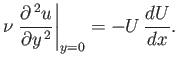
The boundary layer equations, (8.110)-(8.113), take the form
subject to the boundary conditions
Furthermore, it follows from Equations (8.140), (8.142), and (8.143) that
 |
(8.144) |
The previous expression can be thought of as an alternative form of Equation (8.143).
As we saw in Section 8.4, the boundary layer equations can be solved exactly when  takes the special form
 .
However, in the general case, we must resort to approximation methods.
.
However, in the general case, we must resort to approximation methods.
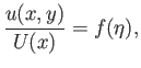
Following Pohlhausen (Schlichting 1987), let us assume that
 |
(8.145) |
where
 , and
, and
 .
In particular, suppose that
.
In particular, suppose that
![$\displaystyle f(\eta)=\left\{\begin{array}{lcl} a+b\,\eta+c\,\eta^{\,2}+d\,\eta...
...\,4}&\mbox{\hspace{1cm}}&0\leq\eta\leq 1\\ [0.5ex] 1&&\eta>1\end{array}\right.,$](img3155.png) |
(8.146) |
where  ,
,  ,
,  ,
,  , and
, and  are constants. This expression automatically satisfies the boundary condition (8.141).
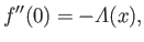
Moreover, the boundary conditions (8.142) and (8.144) imply that
are constants. This expression automatically satisfies the boundary condition (8.141).
Moreover, the boundary conditions (8.142) and (8.144) imply that  , and
, and
 |
(8.147) |
where
 , and
, and
 |
(8.148) |
Finally, let us assume that  ,
,  , and
, and  are continuous at
  : that is,
These constraints corresponds to the reasonable requirements that the
velocity, vorticity, and viscous stress tensor, respectively, be continuous across the layer.
Given that
, Equations (8.146), (8.147), and (8.149)-(8.151) yield
 |
(8.152) |
for
 ,
where
,
where
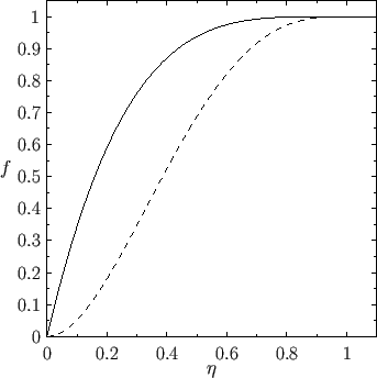
Thus, the tangential velocity profile across the layer is a function of a single parameter,
 , which is
termed the Pohlhausen parameter. The behavior of this profile is illustrated in Figure 8.13. Note that, under normal
circumstances,
the Pohlhausen parameter must lie in the range
, which is
termed the Pohlhausen parameter. The behavior of this profile is illustrated in Figure 8.13. Note that, under normal
circumstances,
the Pohlhausen parameter must lie in the range
 . For
. For
 , the
profile is such that
, the
profile is such that  for some
  , which is not possible in a steady-state solution. On the
other hand, for
, which is not possible in a steady-state solution. On the
other hand, for
 , the profile is such that
  , which implies flow reversal close to the wall.
As we have seen, flow reversal is indicative of separation. Indeed, the separation
point,
, which implies flow reversal close to the wall.
As we have seen, flow reversal is indicative of separation. Indeed, the separation
point,  , corresponds to
 . Expression (8.152) is only an approximation, because
it satisfies some, but not all, of the boundary conditions satisfied by the true velocity profile. For instance, differentiation
of Equation (8.140) with respect to
. Expression (8.152) is only an approximation, because
it satisfies some, but not all, of the boundary conditions satisfied by the true velocity profile. For instance, differentiation
of Equation (8.140) with respect to  reveals that
 , which is not the case for expression (8.152).
Figure:
Pohlhausen velocity profiles for
 (solid curve) and
(dashed curve).
(solid curve) and
(dashed curve).
 |
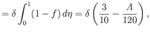
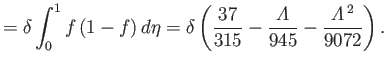
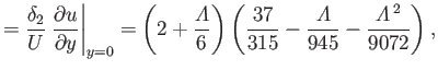
It follows from Equations (8.115), (8.116), and (8.152)-(8.154) that
Furthermore,
 |
(8.157) |
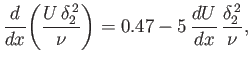
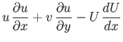
The von Kármán momentum integral, (8.117), can be rearranged to give
 |
(8.158) |
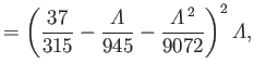
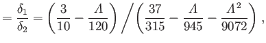
Defining
 |
(8.159) |
we obtain
![$\displaystyle U\,\frac{d}{dx}\!\left(\frac{\lambda}{dU/dx}\right) = 2\left[F_2(\lambda)-\lambda\left\{2+F_1(\lambda)\right\}\right] = F(\lambda),$](img3188.png) |
(8.160) |
where
It is generally necessary to integrate Equation (8.158) from the stagnation point at the front of the obstacle, through the
point of maximum tangential velocity, to the separation point on the back side of the obstacle. At the
stagnation point we have  and
and
 , which implies that
 . Furthermore, at the point of maximum tangential velocity we have
 and
and  , which implies that
 . Finally, as we have already seen,
at the separation point, which implies, from Equation (8.161), that
. Finally, as we have already seen,
at the separation point, which implies, from Equation (8.161), that
 .
.
Figure:
The function
 (solid curve) and the linear function
 (dashed line).
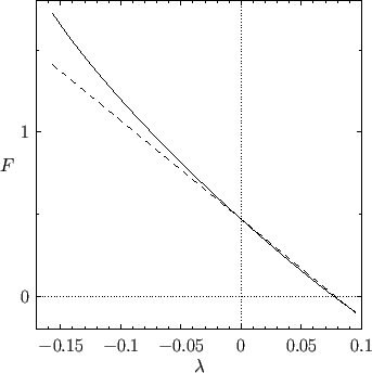 |
As was first pointed out by Walz (Schlichting 1987), and is illustrated in Figure 8.14, it is a fairly good approximation to
replace
by the linear function
for  in the physically relevant range. The approximation is
particularly accurate on the front side of the obstacle (where
in the physically relevant range. The approximation is
particularly accurate on the front side of the obstacle (where  ). Making use of this
approximation, Equations (8.159) and (8.160) reduce to
the linear differential equation
). Making use of this
approximation, Equations (8.159) and (8.160) reduce to
the linear differential equation
 |
(8.165) |
which can be integrated to give
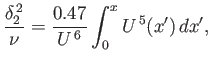 |
(8.166) |
assuming that the stagnation point corresponds to  . It follows that
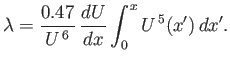 |
(8.167) |
Recall that the separation point corresponds to  , where
 .
.
Suppose that  , which corresponds to uniform flow over a flat plate. (See Section 8.5.)
It follows from Equations (8.166) and (8.167) that
, which corresponds to uniform flow over a flat plate. (See Section 8.5.)
It follows from Equations (8.166) and (8.167) that
 |
(8.168) |
where
 , and
, and  . Moreover, according to Equations (8.148) and (8.162),
 and
and
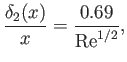
 . Hence, the displacement width of the boundary layer becomes
 |
(8.169) |
This approximate result compares very favorably with the exact result, (8.73).
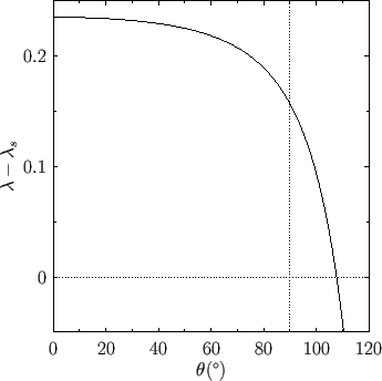
Figure:
The function
 for flow around a circular cylinder.
 |
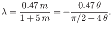
Suppose that
 and
and
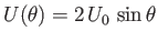 , which corresponds to uniform transverse flow around a circular cylinder of radius
. (See Section 8.8.) Equation (8.167) yields
, which corresponds to uniform transverse flow around a circular cylinder of radius
. (See Section 8.8.) Equation (8.167) yields
 |
(8.170) |
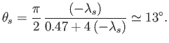
Figure 8.15 shows
determined from the previous formula. It can be seen that
 when
when
 . In other words, the separation point is located
  from the stagnation point at
the front of the cylinder. This suggests that the low pressure wake behind the cylinder is almost as wide as the
cylinder itself, and that the associated form drag is comparatively large.
from the stagnation point at
the front of the cylinder. This suggests that the low pressure wake behind the cylinder is almost as wide as the
cylinder itself, and that the associated form drag is comparatively large.
Figure 8.16:
Flow over the back surface of a semi-infinite wedge.
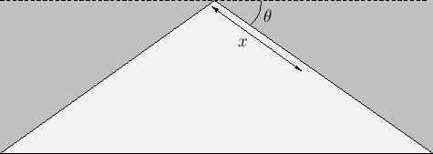 |
Suppose, finally, that
 . If
. If  is negative then, as illustrated in Figure 8.16, this corresponds to uniform flow over the back surface of a semi-infinite
wedge whose angle of dip is
is negative then, as illustrated in Figure 8.16, this corresponds to uniform flow over the back surface of a semi-infinite
wedge whose angle of dip is
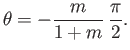 |
(8.171) |
(See Section 8.4.)
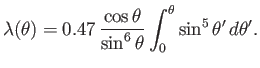
It follows from Equation (8.167) that
 |
(8.172) |
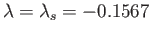
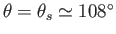
We expect boundary layer separation on the back surface of the wedge when
 . This corresponds to
 , where
 |
(8.173) |
Hence, boundary layer separation can be prevented by making the wedge's angle of
dip sufficiently shallow: that is, by streamlining the wedge, which has the effect of reducing the deceleration of the
flow on the wedge's back surface.
The critical value of
(i.e.,
 ) at which separation occurs in our approximate solution is
very similar to the critical value of
(i.e.,
) at which separation occurs in our approximate solution is
very similar to the critical value of
(i.e.,
 ) at which the exact self-similar solutions described in Section 8.4
can no longer be found. This suggests that the absence of self-similar solutions for
) at which the exact self-similar solutions described in Section 8.4
can no longer be found. This suggests that the absence of self-similar solutions for  is related to
boundary layer separation.
is related to
boundary layer separation.
Next: Exercises
Up: Incompressible Boundary Layers
Previous: Criterion for Boundary Layer
Richard Fitzpatrick
2016-03-31


![$\displaystyle = 2\left(\frac{37}{315}-\frac{{\mit\Lambda}}{945}-\frac{{\mit\Lam...
...{1}{120}\right){\mit\Lambda}^{\,2}+ \frac{2}{9072}\,{\mit\Lambda}^{\,3}\right].$](img3196.png)