


Next: An example 2-d Poisson
Up: Poisson's equation
Previous: 2-d problem with Neumann
The fast Fourier transform
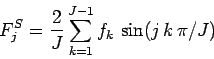
The method outlined in Sect. 5.7 for solving Poisson's equation in 2-d with
simple Dirichlet boundary conditions in the  -direction requires us to perform very many
Fourier-sine transforms:
-direction requires us to perform very many
Fourier-sine transforms:
 |
(169) |
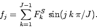
for  , and inverse Fourier-sine transforms:
 |
(170) |
Here,  is the value of
  at
at  .
Thus, Eq. (169) is analogous to Eqs. (153) and (156), whereas
Eq. (170) can be used to reconstruct the
.
Thus, Eq. (169) is analogous to Eqs. (153) and (156), whereas
Eq. (170) can be used to reconstruct the  from the
  .
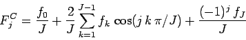
Likewise, the
method outlined in Sect. 5.8 for solving Poisson's equation in 2-d with
simple Neumann boundary conditions in the -direction requires us to perform very many
Fourier-cosine transforms:
.
Likewise, the
method outlined in Sect. 5.8 for solving Poisson's equation in 2-d with
simple Neumann boundary conditions in the -direction requires us to perform very many
Fourier-cosine transforms:
 |
(171) |
for , and inverse Fourier-cosine transforms:
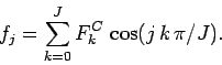 |
(172) |
Unfortunately, performing such transforms directly requires  arithmetic
operations, which means that they are extremely expensive in terms of cpu resources.
There is, however, an ingenious
algorithm for performing Fourier transforms which only takes
arithmetic
operations, which means that they are extremely expensive in terms of cpu resources.
There is, however, an ingenious
algorithm for performing Fourier transforms which only takes  arithmetic
operations [which is much less than operations when
arithmetic
operations [which is much less than operations when  is large].
This algorithm is known as the fast Fourier transform or FFT.35
is large].
This algorithm is known as the fast Fourier transform or FFT.35
The details of the FFT algorithm lie beyond the scope of this course. Roughly speaking,
the algorithm works by building up the transform in stages using
2, 4, 8, 16, etc. grid-points. In this course, we shall employ the
best-known publicly available FFT library,
called the fftw library,36 to perform all of our Fourier-sine and -cosine transforms.
Unfortunately, the fftw library does not directly calculate Fourier-sine and
-cosine transforms.37 Instead, it calculates complex Fourier transforms:
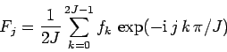 |
(173) |
for  , and complex inverse Fourier transforms:
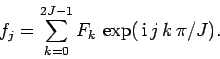 |
(174) |
Note that and  are periodic in
  with period
  .
Note, further, that the data-sets associated with complex Fourier transforms contain twice as many
elements as the data-sets associated with sine and cosine transforms.
However, we can easily convert a sine or cosine transform into a complex transform by extending
its data-set. Thus, for a sine transform we write:
.
Note, further, that the data-sets associated with complex Fourier transforms contain twice as many
elements as the data-sets associated with sine and cosine transforms.
However, we can easily convert a sine or cosine transform into a complex transform by extending
its data-set. Thus, for a sine transform we write:
for  , in which case
 |
(177) |
Likewise, for a cosine transform we write:
for , in which case
 |
(180) |
Listed below are a set of wrapper routines which employ the fftw library to
perform Fourier-sine and -cosine transforms.
// FFT.cpp

// Set of functions to calculate Fourier-cosine and -sine transforms
// of real data using fftw Fast-Fourier-Transform library.
// Input/ouput arrays are assumed to be of extent J+1.
// Uses version 2 of fftw library (incompatible with vs 3).

#include <fftw.h>
#include <blitz/array.h>

using namespace blitz;

// Calculates Fourier-cosine transform of array f in array F
void fft_forward_cos (Array<double,1> f, Array<double,1>& F)
{
  // Find J. Declare local arrays.
  int J = f.extent(0) - 1;
  int N = 2 * J;
  fftw_complex ff[N], FF[N];

  // Load and extend data
  c_re (ff[0]) = f(0); c_im (ff[0]) = 0.;
  c_re (ff[J]) = f(J); c_im (ff[J]) = 0.;
  for (int j = 1; j < J; j++)
    {
      c_re (ff[j]) = f(j); c_im (ff[j]) = 0.;
      c_re (ff[2*J-j]) = f(j); c_im (ff[2*J-j]) = 0.;
    }

  // Call fftw routine
  fftw_plan p = fftw_create_plan (N, FFTW_FORWARD, FFTW_ESTIMATE);
  fftw_one (p, ff, FF);
  fftw_destroy_plan (p);

  // Unload data
  F(0) = c_re (FF[0]); F(J) = c_re (FF[J]);
  for (int j = 1; j < J; j++)
    {
      F(j) = 2. * c_re (FF[j]);
    }

  // Normalize data
  F /= 2. * double (J);
}

// Calculates inverse Fourier-cosine transform of array F in array f
void fft_backward_cos (Array<double,1> F, Array<double,1>& f)
{
  // Find J. Declare local arrays.
  int J = f.extent(0) - 1;
  int N = 2 * J;
  fftw_complex ff[N], FF[N];

  // Load and extend data
  c_re (FF[0]) = F(0); c_im (FF[0]) = 0.;
  c_re (FF[J]) = F(J); c_im (FF[J]) = 0.;
  for (int j = 1; j < J; j++)
    {
      c_re (FF[j]) = F(j) / 2.; c_im (FF[j]) = 0.;
      FF[2*J-j] = FF[j];
    }

  // Call fftw routine
  fftw_plan p = fftw_create_plan (N, FFTW_BACKWARD, FFTW_ESTIMATE);
  fftw_one (p, FF, ff);
  fftw_destroy_plan (p);

  // Unload data
  f(0) = c_re (ff[0]); f(J) = c_re (ff[J]);
  for (int j = 1; j < J; j++)
    {
      f(j) = c_re (ff[j]);
    }
}

// Calculates Fourier-sine transform of array f in array F
void fft_forward_sin (Array<double,1> f, Array<double,1>& F)
{
  // Find J. Declare local arrays.
  int J = f.extent(0) - 1;
  int N = 2 * J;
  fftw_complex ff[N], FF[N];

  // Load and extend data
  c_re (ff[0]) = 0.; c_im (ff[0]) = 0.;
  c_re (ff[J]) = 0.; c_im (ff[J]) = 0.;
  for (int j = 1; j < J; j++)
    {
      c_re (ff[j]) = f(j); c_im (ff[j]) = 0.;
      c_re (ff[2*J-j]) = - f(j); c_im (ff[2*J-j]) = 0.;
    }

  // Call fftw routine
  fftw_plan p = fftw_create_plan (N, FFTW_FORWARD, FFTW_ESTIMATE);
  fftw_one (p, ff, FF);
  fftw_destroy_plan (p);

  // Unload data
  F(0) = 0.; F(J) = 0.;
  for (int j = 1; j < J; j++)
    {
      F(j) = - 2. * c_im (FF[j]);
    }

  // Normalize data
  F /= 2. * double (J);
}

// Calculates inverse Fourier-sine transform of array F in array f
void fft_backward_sin (Array<double,1> F, Array<double,1>& f)
{
  // Find J. Declare local arrays.
  int J = f.extent(0) - 1;
  int N = 2 * J;
  fftw_complex ff[N], FF[N];

  // Load and extend data
  c_re (FF[0]) = 0.; c_im (FF[0]) = 0.;
  c_re (FF[J]) = 0.; c_im (FF[J]) = 0.;
  for (int j = 1; j < J; j++)
    {
      c_re (FF[j]) = 0.; c_im (FF[j]) = - F(j) / 2.;
      c_re (FF[2*J-j]) = 0.; c_im (FF[2*J-j]) = F(j) / 2.;
    }

  // Call fftw routine
  fftw_plan p = fftw_create_plan (N, FFTW_BACKWARD, FFTW_ESTIMATE);
  fftw_one (p, FF, ff);
  fftw_destroy_plan (p);

  // Unload data
  f(0) = 0.; f(J) = 0.;
  for (int j = 1; j < J; j++)
    {
      f(j) = c_re (ff[j]);
    }
}
Next: An example 2-d Poisson
Up: Poisson's equation
Previous: 2-d problem with Neumann
Richard Fitzpatrick
2006-03-29