An example solution of Poisson's equation in 1-d

Next: 2-d problem with Dirichlet Up: Poisson's equation Previous: An example 1-d Poisson

An example solution of Poisson's equation in 1-d

Let us now solve Poisson's equation in one dimension, with mixed boundary conditions, using the finite difference technique discussed above. We seek the solution of

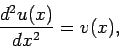$\begin{displaymath} \frac{d^2 u(x)}{dx^2} = v(x), \end{displaymath}$

(142)

in the region 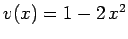$0\leq x\leq 1$ , with $v(x) = 1 - 2\,x^2$ . The boundary conditions at

and

take the mixed form specified in Eqs. (132) and (133). Of course, we can solve this problem analytically. In fact,

$\begin{displaymath} u(x) = g + h\,x + \frac{x^2}{2} - \frac{x^4}{6}, \end{displaymath}$

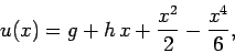(143)

where

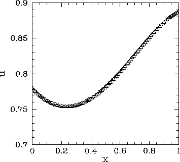
$\displaystyle g$	$\textstyle =$	$\displaystyle \frac{\gamma_l\,(\alpha_h+\beta_h) - \beta_l\,[\gamma_h-(\alpha_h+\beta_h)/3]} {\alpha_l\,\alpha_h + \alpha_l\,\beta_h-\beta_l\,\alpha_h},$	(144)
$\displaystyle h$	$\textstyle =$	$\displaystyle \frac{ \alpha_l\,[\gamma_h-(\alpha_h+\beta_h)/3]-\gamma_l\,\alpha_h} {\alpha_l\,\alpha_h + \alpha_l\,\beta_h-\beta_l\,\alpha_h}.$	(145)

Figure 62 shows a comparison between the analytic and finite difference solutions for

. It can be seen that the finite difference solution mirrors the analytic solution almost exactly.

**Figure 62:** Solution of Poisson's equation in one dimension with 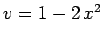$v=1-2\,x^2$ , $\alpha _l = 1$ , $\beta _l=-1$ , $\gamma _l=1$ , $\alpha _h=1$ , $\beta _h=1$ , and $\gamma _h=1$ . The dotted curve (obscured) shows the analytic solution, whereas the open triangles show the finite difference solution for .
$\begin{figure} \epsfysize =3in \centerline{\epsffile{p1d.eps}} \end{figure}$

Next: 2-d problem with Dirichlet Up: Poisson's equation Previous: An example 1-d Poisson

Richard Fitzpatrick 2006-03-29