Oscillation of an Elastic Sheet
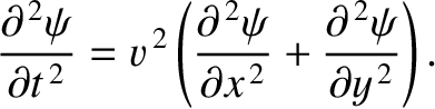
A straightforward generalization of the analysis of Section 4.3 reveals that the transverse oscillation of a uniform
elastic sheet, stretched over a rigid frame, is governed by the two-dimensional wave equation (Pain 1999)
 |
(7.14) |
Here,
 is the sheet's transverse (i.e., in the
  -direction)
displacement,
-direction)
displacement,
 the characteristic speed of elastic waves on the sheet,
  the tension, and
  the
mass per unit area. In equilibrium, the sheet is assumed to lie in the
the
mass per unit area. In equilibrium, the sheet is assumed to lie in the  -
- plane. The boundary condition is that
 at the rigid frame.
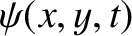
Figure 7.4:
Density plot illustrating the spatial variation of the  ,
,  normal mode of a rectangular elastic sheet with
 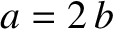 . Dark/light
regions indicate positive/negative displacements.
. Dark/light
regions indicate positive/negative displacements.
|
|
Suppose that the frame is rectangular, extending from  to
to  , and from
  to
to  . Let us
search for a normal mode of the form
. Let us
search for a normal mode of the form
 |
(7.15) |
Substitution into Equation (7.14) yields
 |
(7.16) |
subject to the boundary conditions
 . Let us search for a separable solution of the form
 |
(7.17) |
Such a solution satisfies the boundary conditions provided
 . It follows that
 |
(7.18) |
The only way that the preceding equation can be satisfied at all and is if
where
 and
and
 are positive constants. (The constants have to be positive, rather than negative, to give oscillatory
solutions that are capable of satisfying the boundary conditions.)
Appropriate solutions of Equations (7.19) and (7.20) are
where
are positive constants. (The constants have to be positive, rather than negative, to give oscillatory
solutions that are capable of satisfying the boundary conditions.)
Appropriate solutions of Equations (7.19) and (7.20) are
where  and
and  are arbitrary constants. These solutions automatically satisfy the
boundary conditions
are arbitrary constants. These solutions automatically satisfy the
boundary conditions
 . The boundary conditions
 are satisfied provided
where
are satisfied provided
where  and
and  are positive integers. Thus, the normal modes of a rectangular elastic sheet, which are indexed
by the mode numbers and , take the form
are positive integers. Thus, the normal modes of a rectangular elastic sheet, which are indexed
by the mode numbers and , take the form
 |
(7.26) |
where
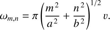 |
(7.27) |
Here,  and
and
 are arbitrary constants. Because Equation (7.14) is linear, its solutions are superposable. Hence,
the most general solution is a superposition of all of the normal modes; that is,
are arbitrary constants. Because Equation (7.14) is linear, its solutions are superposable. Hence,
the most general solution is a superposition of all of the normal modes; that is,
 |
(7.28) |
The amplitudes , and the phase angles
 , are determined by the initial conditions. (See Exercise 4.) Figure 7.4 illustrates
the spatial variation of the , normal mode of a rectangular elastic sheet with .
, are determined by the initial conditions. (See Exercise 4.) Figure 7.4 illustrates
the spatial variation of the , normal mode of a rectangular elastic sheet with .
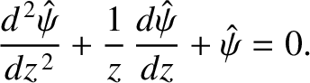
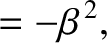
Figure 7.5:
The Bessel function  .
.
|
|
Suppose that an elastic sheet is stretched over a circular frame of radius  . Defining the radial cylindrical coordinate
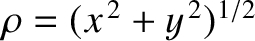 ,
where
,
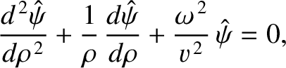
where  corresponds to the location of the frame, the axisymmetric oscillations of the sheet are governed by the
cylindrical wave equation (see Section 7.4)
corresponds to the location of the frame, the axisymmetric oscillations of the sheet are governed by the
cylindrical wave equation (see Section 7.4)
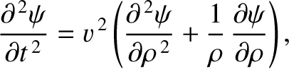 |
(7.29) |
subject to the boundary condition at . Let us search for a normal mode of the form
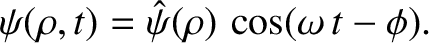 |
(7.30) |
Substitution into Equation (7.29) yields
 |
(7.31) |
subject to the boundary condition
 . Let us define the scaled radial coordinate
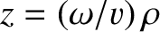 . When
written in terms of this new coordinate, the previous equation transforms to
. When
written in terms of this new coordinate, the previous equation transforms to
 |
(7.32) |
This well-known equation is called Bessel's equation (of degree zero), and has the standard solution (that is well-behaved at  ) (Abramowitz and Stegun 1965)
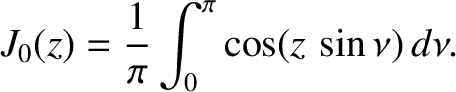 |
(7.33) |
Here, is termed a Bessel function (of degree zero), and is
plotted in Figure 7.5. It can be seen that the function is broadly similar to a cosine function,
except that its zeros are not quite evenly spaced, and its amplitude gradually decreases as increases. The first few values of at which  are
listed in Table 7.1. Let the
are
listed in Table 7.1. Let the  th zero be located at
  . In order to satisfy the boundary condition, we
require that
. In order to satisfy the boundary condition, we
require that
 . Hence, the axisymmetric normal modes of an elastic sheet, stretched over
a circular frame of radius , are indexed by the mode number (which is a positive integer), and take the form
. Hence, the axisymmetric normal modes of an elastic sheet, stretched over
a circular frame of radius , are indexed by the mode number (which is a positive integer), and take the form
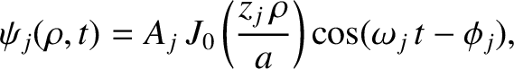 |
(7.34) |
where
 |
(7.35) |
and  ,
,  are arbitrary constants. Figure 7.6 illustrates the spatial variation of the
  normal mode.
Table: 7.1
First few zeros of the Bessel function . Source: Abramowitz and Stegun 1965.
|
 |
|
|
| |
|
|
|
| 1 |
2.40482 |
6 |
18.07106 |
| 2 |
5.52007 |
7 |
21.21163 |
| 3 |
8.65372 |
8 |
24.35247 |
| 4 |
11.79153 |
9 |
27.49347 |
| 5 |
14.93091 |
10 |
30.63460 |
|
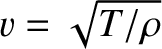
Figure 7.6:
Density plot illustrating the spatial variation of the normal mode of a circular elastic sheet of radius . Dark/light
regions indicate large/small displacement amplitudes.
|
|
![\includegraphics[width=1\textwidth]{Chapter07/fig7_04.eps}](img1871.png)


![\includegraphics[width=0.8\textwidth]{Chapter07/fig7_06.eps}](img1923.png)

![\includegraphics[width=0.8\textwidth]{Chapter07/fig7_05.eps}](img1906.png)