Next: Longitudinal Waves on Thin Up: Longitudinal Standing Waves Previous: Introduction Contents
 identical masses
  that are free to slide in one dimension over a frictionless
horizontal surface. Suppose that the masses are coupled to their immediate neighbors via
identical light springs of unstretched length
that are free to slide in one dimension over a frictionless
horizontal surface. Suppose that the masses are coupled to their immediate neighbors via
identical light springs of unstretched length  , and force constant
  . (Here, we employ the symbol to
denote the spring force constant, rather than
. (Here, we employ the symbol to
denote the spring force constant, rather than  , because is already being used to denote wavenumber.) Let
  measure distance along the array (from the left to the right). If the array is in its equilibrium state then the -coordinate
of the
measure distance along the array (from the left to the right). If the array is in its equilibrium state then the -coordinate
of the  th mass is
  , for
, for  . Consider longitudinal oscillations
of the masses. Namely, oscillations for which the -coordinate of the th mass is
. Consider longitudinal oscillations
of the masses. Namely, oscillations for which the -coordinate of the th mass is
 |
(5.1) |
 represents longitudinal displacement from equilibrium. It is assumed that all of the displacements are relatively small; that is,
 , for
.
, for
.
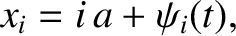
Consider the equation of motion of the th mass. See Figure 5.1. The
extensions of the springs to the immediate left and right of the mass are
 and
and
 , respectively. Thus, the -directed
forces that these springs exert on the mass are
, respectively. Thus, the -directed
forces that these springs exert on the mass are
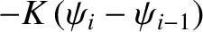 and
and
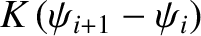 , respectively. The mass's equation of
motion therefore becomes
, respectively. The mass's equation of
motion therefore becomes
 . Because there is nothing special about the th mass, the
preceding equation is assumed to hold for all masses; that is, for .
Equation (5.2), which governs the longitudinal oscillations of a linear array of spring-coupled masses, is analogous in
form to Equation (4.8), which governs the transverse oscillations
of a beaded string. This observation suggests that longitudinal and transverse waves in discrete dynamical systems (i.e., systems with a finite number of degrees
of freedom)
can be described using the same mathematical equations.
. Because there is nothing special about the th mass, the
preceding equation is assumed to hold for all masses; that is, for .
Equation (5.2), which governs the longitudinal oscillations of a linear array of spring-coupled masses, is analogous in
form to Equation (4.8), which governs the transverse oscillations
of a beaded string. This observation suggests that longitudinal and transverse waves in discrete dynamical systems (i.e., systems with a finite number of degrees
of freedom)
can be described using the same mathematical equations.
![\includegraphics[width=1\textwidth]{Chapter05/fig5_02.eps}](img1128.png) |
We can interpret the quantities  and
and
 , that appear
in the equations of motion for
, that appear
in the equations of motion for  and
and  , respectively, as the longitudinal displacements of
the left and right extremities of springs attached to the outermost masses in such a manner as to form the left and right boundaries of the array.
The respective equilibrium positions of these extremities are
, respectively, as the longitudinal displacements of
the left and right extremities of springs attached to the outermost masses in such a manner as to form the left and right boundaries of the array.
The respective equilibrium positions of these extremities are  and
and
 .
The end displacements, and
, must be prescribed, otherwise Equations (5.2)
do not constitute a complete set of equations. In other words, there are more unknowns than equations.
The particular choice of and
depends on the nature of the physical
boundary conditions at the two ends of the array. Suppose that the
left extremity of the leftmost spring is anchored in an
immovable wall. This implies that
.
The end displacements, and
, must be prescribed, otherwise Equations (5.2)
do not constitute a complete set of equations. In other words, there are more unknowns than equations.
The particular choice of and
depends on the nature of the physical
boundary conditions at the two ends of the array. Suppose that the
left extremity of the leftmost spring is anchored in an
immovable wall. This implies that  ; that is, the left extremity of the
spring cannot move. Suppose, on the other hand, that the left extremity of the leftmost spring is not attached to anything. In this case, there is no reason for the spring
to become extended, which implies that
; that is, the left extremity of the
spring cannot move. Suppose, on the other hand, that the left extremity of the leftmost spring is not attached to anything. In this case, there is no reason for the spring
to become extended, which implies that
 . In other words, if the left
end of the array is fixed (i.e., attached to an immovable object) then , and if the left end is
free (i.e., not attached to anything) then
. Likewise, if the right end of the array
is fixed then
. In other words, if the left
end of the array is fixed (i.e., attached to an immovable object) then , and if the left end is
free (i.e., not attached to anything) then
. Likewise, if the right end of the array
is fixed then
 , and if the right end is free then
 .
.
Suppose, for the sake of argument, that the left end of the array is
free, and the right end is fixed. It follows that
, and
.
Let us search for normal
modes of the general form
 ,
,  ,
,  , and
, and  are constants.
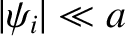
The preceding expression automatically satisfies the boundary condition
. This follows because
and
are constants.
The preceding expression automatically satisfies the boundary condition
. This follows because
and  , and, consequently,
![$\cos[k\,(x_0-a/2)]=\cos(-k\,a/2)=\cos(k\,a/2)=\cos[k\,(x_1-a/2)]$](img1139.png) . The other boundary condition,
, is satisfied provided
. The other boundary condition,
, is satisfied provided
![$\displaystyle \cos[k\,(x_{N+1}-a/2)] = \cos[(N+1/2)\,k\,a] = 0,$](img1140.png) |
(5.4) |
 is an integer. As before, the imposition of the boundary conditions
causes a quantization of the possible mode wavenumbers. (See Section 4.2.)
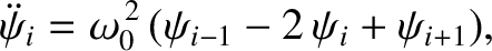
Finally, substitution of Equation (5.3) into Equation (5.2) gives the
dispersion relation [cf., Equation (4.16)]
is an integer. As before, the imposition of the boundary conditions
causes a quantization of the possible mode wavenumbers. (See Section 4.2.)
Finally, substitution of Equation (5.3) into Equation (5.2) gives the
dispersion relation [cf., Equation (4.16)]
It follows, from the preceding analysis, that the longitudinal normal modes of a linear array of spring-coupled masses, the left end of which is free, and the right end fixed, are associated with the following characteristic displacement patterns,
where and the and
and  are arbitrary constants determined by the initial conditions.
Here, the integer indexes the masses, and the mode number indexes the normal modes. It can be
demonstrated that there are only unique normal
modes, corresponding to mode numbers in the range 1 to .
are arbitrary constants determined by the initial conditions.
Here, the integer indexes the masses, and the mode number indexes the normal modes. It can be
demonstrated that there are only unique normal
modes, corresponding to mode numbers in the range 1 to .
![\includegraphics[width=0.9\textwidth]{Chapter05/fig5_03.eps}](img1145.png) |
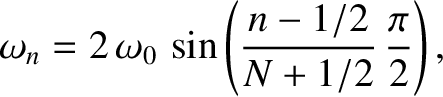
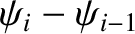
Figures 5.2 and 5.3 display the normal modes and normal
frequencies of a linear array of eight spring-coupled masses, the left end of which is free, and
the right end fixed. The data shown in these figures is obtained from Equations (5.7) and (5.8), respectively, with  .
It can be seen that
normal modes with small wavenumbers—that is,
.
It can be seen that
normal modes with small wavenumbers—that is,  , so that
  —have displacements
that vary in a fairly smooth sinusoidal manner from mass to mass, and oscillation frequencies
that increase approximately linearly with increasing wavenumber.
On the
other hand, normal modes with large wavenumbers—that is,
—have displacements
that vary in a fairly smooth sinusoidal manner from mass to mass, and oscillation frequencies
that increase approximately linearly with increasing wavenumber.
On the
other hand, normal modes with large wavenumbers—that is,
 , so that
  —have
displacements that exhibit large variations from mass to mass, and
oscillation frequencies that do not depend linearly on wavenumber. We conclude that
the longitudinal normal modes of an array of spring-coupled masses have analogous properties
to the transverse normal modes of a beaded string. (See Section 4.2.)
—have
displacements that exhibit large variations from mass to mass, and
oscillation frequencies that do not depend linearly on wavenumber. We conclude that
the longitudinal normal modes of an array of spring-coupled masses have analogous properties
to the transverse normal modes of a beaded string. (See Section 4.2.)
The dynamical system pictured in Figure 5.1 can be used to model the effect of a planar
sound wave (i.e., a longitudinal
oscillation in position that is periodic in space) on a crystal lattice. In this application, the masses represent parallel planes of atoms, the springs represent the interatomic forces acting between these planes, and the
longitudinal oscillations represent the sound wave. Of course, a macroscopic crystal
contains a great many atomic planes, so we would expect to be very large.
However, according to Equations (5.5) and (5.8),
no matter how large becomes,  cannot exceed
  (because cannot exceed ), and
  cannot exceed
 . In other words, there is a minimum wavelength that
a sound wave in a crystal lattice can have, which turns out to be twice the
interplane spacing, and a corresponding maximum oscillation frequency.
For waves whose wavelengths are much greater than the interplane spacing (i.e., ), the dispersion relation (5.6) reduces to
. In other words, there is a minimum wavelength that
a sound wave in a crystal lattice can have, which turns out to be twice the
interplane spacing, and a corresponding maximum oscillation frequency.
For waves whose wavelengths are much greater than the interplane spacing (i.e., ), the dispersion relation (5.6) reduces to
 is a constant that has the dimensions of velocity.
It seems plausible that Equation (5.9) is the dispersion
relation for sound waves in a continuous elastic medium. Let us investigate such waves.
is a constant that has the dimensions of velocity.
It seems plausible that Equation (5.9) is the dispersion
relation for sound waves in a continuous elastic medium. Let us investigate such waves.
![\includegraphics[width=1\textwidth]{Chapter05/fig5_01.eps}](img1121.png)
![$\displaystyle \psi_i(t) = A\,\cos[k\,(x_i-a/2)]\,\cos(\omega\,t-\phi),$](img1138.png)
![$\displaystyle \psi_{n,i} (t) = A_n\,\cos\left[\frac{(n-1/2)\,(i-1/2)}{N+1/2}\,\pi\right]\cos(\omega_n-\phi_n),$](img1143.png)