Next: Normal Modes of Uniform Up: Transverse Standing Waves Previous: Introduction Contents
 identical beads of
mass
identical beads of
mass  are attached to the string in such a manner that they cannot slide along it. Let the beads be equally
spaced a distance
are attached to the string in such a manner that they cannot slide along it. Let the beads be equally
spaced a distance  apart, and let the distance between the first and the last beads and
the neighboring walls also be . See Figure 4.1. Consider transverse
oscillations of the string; that is, oscillations in which the string
moves in a direction perpendicular to its length.
It is assumed that the inertia of the string
is negligible with respect to that of the beads. It follows that the sections of the string
between neighboring beads, and between the outermost beads and the walls,
are straight. (Otherwise, there would be a net tension force acting on the sections, and
they would consequently suffer an infinite acceleration.) In fact, we expect the instantaneous configuration of the string to be a
set of continuous straight-line segments of varying inclinations, as shown in the figure. Finally, assuming that
the transverse displacement of the string is relatively small, it is
reasonable to suppose that each section of the string possesses the
same tension,
apart, and let the distance between the first and the last beads and
the neighboring walls also be . See Figure 4.1. Consider transverse
oscillations of the string; that is, oscillations in which the string
moves in a direction perpendicular to its length.
It is assumed that the inertia of the string
is negligible with respect to that of the beads. It follows that the sections of the string
between neighboring beads, and between the outermost beads and the walls,
are straight. (Otherwise, there would be a net tension force acting on the sections, and
they would consequently suffer an infinite acceleration.) In fact, we expect the instantaneous configuration of the string to be a
set of continuous straight-line segments of varying inclinations, as shown in the figure. Finally, assuming that
the transverse displacement of the string is relatively small, it is
reasonable to suppose that each section of the string possesses the
same tension,  . [See Equation (4.11).]
It is convenient to introduce a Cartesian coordinate system such that  measures distance along the string from the left wall, and
 measures the transverse displacement of the string from its
equilibrium position. See Figure 4.1. Thus, when the string is in its equilibrium position
it runs along the -axis. We can define
measures the transverse displacement of the string from its
equilibrium position. See Figure 4.1. Thus, when the string is in its equilibrium position
it runs along the -axis. We can define
 . Here,
  is the -coordinate of the
closest bead to the left wall,
is the -coordinate of the
closest bead to the left wall,  the
-coordinate of the second-closest bead, et cetera. The -coordinates of the beads
are assumed to remain constant during their transverse oscillations.
We can also define
the
-coordinate of the second-closest bead, et cetera. The -coordinates of the beads
are assumed to remain constant during their transverse oscillations.
We can also define  and
and
 as the -coordinates of the left
and right ends of the string, respectively. Let the transverse displacement
of the
as the -coordinates of the left
and right ends of the string, respectively. Let the transverse displacement
of the  th bead be
  , for
, for 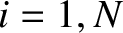 . Because each displacement
can vary independently, we are dealing with an degree of freedom system.
We would, therefore, expect such a system to possess unique normal modes of
oscillation.
. Because each displacement
can vary independently, we are dealing with an degree of freedom system.
We would, therefore, expect such a system to possess unique normal modes of
oscillation.
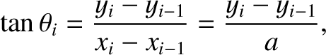
Consider the section of the
string lying between the  th and
  th beads, as shown in Figure 4.2.
Here,
th beads, as shown in Figure 4.2.
Here,
 ,
,  , and
, and
 are the distances of the th, th, and
th beads, respectively,
from the left wall, whereas
are the distances of the th, th, and
th beads, respectively,
from the left wall, whereas  ,
,  , and
, and
 are the corresponding transverse displacements of these beads.
The two sections of the string that are attached to the th
bead subtend angles
are the corresponding transverse displacements of these beads.
The two sections of the string that are attached to the th
bead subtend angles  and
and
 with the -axis, as illustrated
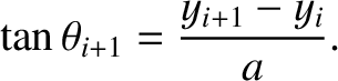
in the figure. Standard trigonometry reveals that
with the -axis, as illustrated
in the figure. Standard trigonometry reveals that
 |
(4.2) |
 |
(4.3) |
 for all —which we shall assume to be
the case, then and
are both small angles. Thus,
we can use the small-angle approximation
for all —which we shall assume to be
the case, then and
are both small angles. Thus,
we can use the small-angle approximation
 . (See Appendix B.) It follows that
Let us find the transverse equation of motion of the th bead. This
bead is subject to two forces: namely, the tensions in the sections
of the string to the left and to the right of it. (Incidentally, we are neglecting any gravitational forces
acting on the beads, compared to the tension forces.) These tensions are of
magnitude , and are directed parallel to the associated string sections, as shown
in Figure 4.2. Thus, the transverse (i.e., -directed) components of
these two tensions are
 and
and
 , respectively.
Hence, the transverse equation of motion of the th bead becomes
, respectively.
Hence, the transverse equation of motion of the th bead becomes
 |
(4.6) |
and
are both small angles, we
can employ the small-angle approximation
 .
It follows that
.
It follows that
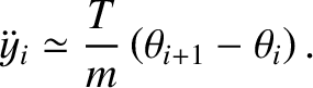 |
(4.7) |
 . Because there is nothing special
about the th bead, we deduce that the preceding equation of motion
applies to all beads; that is, it is valid for . Of course,
the first (
. Because there is nothing special
about the th bead, we deduce that the preceding equation of motion
applies to all beads; that is, it is valid for . Of course,
the first ( ) and last (
 ) beads are special cases, because there
is no bead corresponding to
) beads are special cases, because there
is no bead corresponding to  or
or  . In fact, and
correspond to the left and right ends of the string, respectively. However,
Equation (4.8) still applies to the first and last beads, as long as
we set
. In fact, and
correspond to the left and right ends of the string, respectively. However,
Equation (4.8) still applies to the first and last beads, as long as
we set  and
and  . What we are effectively demanding
is that the two ends of the string, which are attached to the left and right walls, must both have zero transverse
displacement.
. What we are effectively demanding
is that the two ends of the string, which are attached to the left and right walls, must both have zero transverse
displacement.
Incidentally, we can prove that the tensions in the two sections of the string shown in Figure 4.2 must be
equal by considering the longitudinal equation of motion of the th bead. This equation takes the
form
 |
(4.9) |
 and
and  are the, supposedly different, tensions in the sections of the string to the
immediate left and right of the th bead, respectively. We are assuming that the motion
of the beads is purely transverse; that is, all of the are constant in time. Thus, it follows from the
preceding equation that
are the, supposedly different, tensions in the sections of the string to the
immediate left and right of the th bead, respectively. We are assuming that the motion
of the beads is purely transverse; that is, all of the are constant in time. Thus, it follows from the
preceding equation that
 |
(4.10) |
are small then
we can make use of the small-angle approximation
 . (See Appendix B.) Hence, we
obtain
A straightforward extension of this argument reveals that the tension is the same in all sections of the string.
. (See Appendix B.) Hence, we
obtain
A straightforward extension of this argument reveals that the tension is the same in all sections of the string.
Let us search for a normal mode solution to Equation (4.8) that takes the form
where ,
,  ,
,  , and
, and  are constants.
This particular type of solution is such that all of the beads execute transverse simple harmonic oscillations
that are in phase
with one another. See Figure 4.4. Moreover, the oscillations have an amplitude
are constants.
This particular type of solution is such that all of the beads execute transverse simple harmonic oscillations
that are in phase
with one another. See Figure 4.4. Moreover, the oscillations have an amplitude
 that varies sinusoidally along the length of the string (i.e., in the -direction). The pattern of oscillations is thus periodic in space. The spatial repetition period, which is generally termed the wavelength, is
 . [This follows from Equation (4.12) because
 is a periodic function with period
 : i.e.,
 .] The constant
  , which determines the wavelength, is usually referred to as the wavenumber. Thus, a
small wavenumber corresponds to a long wavelength, and vice versa.
The type of solution specified in Equation (4.12) is generally
known as a standing wave. It is a wave because it is periodic
in both space and time. (An oscillation is periodic in time only.) It is
a standing wave, rather than a traveling wave, because the points
of maximum and minimum amplitude oscillation are stationary (in ). See Figure 4.4.
, which determines the wavelength, is usually referred to as the wavenumber. Thus, a
small wavenumber corresponds to a long wavelength, and vice versa.
The type of solution specified in Equation (4.12) is generally
known as a standing wave. It is a wave because it is periodic
in both space and time. (An oscillation is periodic in time only.) It is
a standing wave, rather than a traveling wave, because the points
of maximum and minimum amplitude oscillation are stationary (in ). See Figure 4.4.
Substituting Equation (4.12) into Equation (4.8), we obtain
 |
 |
|
![$\displaystyle ~~\left.+\sin(k\,x_{i+1})\right]\,\cos(\omega\,t-\phi),$](img916.png) |
(4.13) |
![$\displaystyle -\omega^{\,2}\,\sin(k\,x_i)=\omega_0^{\,2}\left(\sin[k\,(x_i-a)] -2\,\sin(k\,x_i)
+\sin[k\,(x_i+a)]\right).$](img917.png) |
(4.14) |
 (see Appendix B), we get
![$\displaystyle -\omega^{\,2}\,\sin(k\,x_i)=\omega_0^{\,2}\left[\cos(k\,a)-2+\cos(k\,a)\right]\sin(k\,x_i),$](img919.png) |
(4.15) |
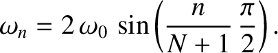
 . (See Appendix B.) An expression, such as Equation (4.16), that determines the angular frequency,
  , of
a wave in terms of its wavenumber, , is generally termed a dispersion relation.
, of
a wave in terms of its wavenumber, , is generally termed a dispersion relation.
The solution (4.12) is only physical provided
 . In other words,
provided the two ends of the string remain stationary. The first constraint
is automatically satisfied, because . See Equation (4.1). The second constraint
implies that
. In other words,
provided the two ends of the string remain stationary. The first constraint
is automatically satisfied, because . See Equation (4.1). The second constraint
implies that
![$\displaystyle \sin(k\,x_{N+1}) = \sin[(N+1)\,k\,a] = 0.$](img923.png) |
(4.17) |
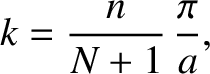
 is known as a mode number. A small mode number translates to a small wavenumber, and, hence, to a
long wavelength, and vice versa. We conclude that the possible wavenumbers, , of the normal modes of the system are
quantized such that they are integer multiples of
is known as a mode number. A small mode number translates to a small wavenumber, and, hence, to a
long wavelength, and vice versa. We conclude that the possible wavenumbers, , of the normal modes of the system are
quantized such that they are integer multiples of
![$\pi/[(N+1)\,a]$](img925.png) .
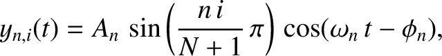
Thus, the th normal mode is
associated with the characteristic pattern of bead displacements
where
Here, the integer indexes the beads, whereas the mode number indexes the normal modes. Furthermore,
.
Thus, the th normal mode is
associated with the characteristic pattern of bead displacements
where
Here, the integer indexes the beads, whereas the mode number indexes the normal modes. Furthermore,
 and
and  are arbitrary constants determined by the initial conditions.
Of course, is the peak amplitude of the th normal mode, whereas
is the associated phase angle.
are arbitrary constants determined by the initial conditions.
Of course, is the peak amplitude of the th normal mode, whereas
is the associated phase angle.
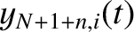
How many unique normal modes does the system possess? At first sight, it
might seem that there are an infinite number of normal modes, corresponding to the
infinite number of possible values that the integer can take. However, this is not
the case. For instance, if  or
or  then all of the
  are zero.
Clearly, these cases are not real normal modes. Moreover, it can be
demonstrated that
are zero.
Clearly, these cases are not real normal modes. Moreover, it can be
demonstrated that
 |
 |
(4.21) |
 |
 |
(4.22) |
 and
and
 , as well as
 |
 |
(4.23) |
 |
 |
(4.24) |
 and
and
 . We,
thus, conclude that only those normal modes that have in the
range
. We,
thus, conclude that only those normal modes that have in the
range  to correspond to unique modes. Modes with values lying outside
this range are either null modes, or modes that are identical to other modes
with values lying within the prescribed range. It follows that
there are unique normal modes of the form (4.19). Hence, given that we are dealing with an degree of
freedom system, which we would expect to only possess unique normal modes, we can be sure that we have found all the normal modes.
to correspond to unique modes. Modes with values lying outside
this range are either null modes, or modes that are identical to other modes
with values lying within the prescribed range. It follows that
there are unique normal modes of the form (4.19). Hence, given that we are dealing with an degree of
freedom system, which we would expect to only possess unique normal modes, we can be sure that we have found all the normal modes.
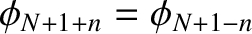
![\includegraphics[width=1\textwidth]{Chapter04/fig4_03.eps}](img946.png) |
Figure 4.3 illustrates the spatial variation of the normal modes of a beaded string possessing eight
beads. That is, an  system. It can be seen that the low-—that is, long-wavelength—modes cause the string to oscillate in a
fairly smoothly-varying (in ) sine wave pattern. On the other hand, the high-—that is, short-wavelength—modes cause the string to oscillate in a
rapidly-varying zig-zag pattern that bears little resemblance to a sine wave.
The crucial distinction between the two different types of mode is that the
wavelength of the oscillation (in the -direction) is much larger
than the bead spacing in the former case, while it is similar to
the bead spacing in the latter. For instance,
system. It can be seen that the low-—that is, long-wavelength—modes cause the string to oscillate in a
fairly smoothly-varying (in ) sine wave pattern. On the other hand, the high-—that is, short-wavelength—modes cause the string to oscillate in a
rapidly-varying zig-zag pattern that bears little resemblance to a sine wave.
The crucial distinction between the two different types of mode is that the
wavelength of the oscillation (in the -direction) is much larger
than the bead spacing in the former case, while it is similar to
the bead spacing in the latter. For instance,
 for the
  mode,
mode,
 for the
  mode, but
 for the
  mode.
mode.
![\includegraphics[width=0.9\textwidth]{Chapter04/fig4_04.eps}](img954.png) |
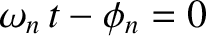
Figure 4.5 displays the temporal variation of the normal mode of
an beaded string. It can be seen
that the beads oscillate in phase with one another. In other words, they all attain their maximal
transverse displacements, and pass through zero displacement, simultaneously.
Moreover, the mid-way point of the string always remains stationary. Such a point is
known as a node. The normal mode has two nodes (counting the
stationary points at each end of the string as nodes), the
mode has three nodes, the  mode four nodes, et cetera. In fact, the existence
of nodes is one of the distinguishing features of a standing wave.
mode four nodes, et cetera. In fact, the existence
of nodes is one of the distinguishing features of a standing wave.
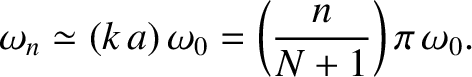
Figure 4.5 shows the normal frequencies of an
beaded string plotted as a function of the normalized wavenumber. Recall that, for an
system,
the relationship between the normalized wavenumber,  , and the
mode number, , is
, and the
mode number, , is
 .
It can be seen that the angular frequency increases as the wavenumber
increases, which implies that shorter wavelength modes have
higher oscillation frequencies. The dependence of the angular frequency
on the normalized wavenumber, , is approximately linear when
.
It can be seen that the angular frequency increases as the wavenumber
increases, which implies that shorter wavelength modes have
higher oscillation frequencies. The dependence of the angular frequency
on the normalized wavenumber, , is approximately linear when 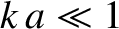 . Indeed, it can be seen from Equation (4.20) that if then the small-angle approximation
yields a linear dispersion relation
of the form
. Indeed, it can be seen from Equation (4.20) that if then the small-angle approximation
yields a linear dispersion relation
of the form
) have approximately linear dispersion
relations in which their angular frequencies are directly proportional
to their mode numbers. However, it is evident from the figure that this linear relationship
breaks down as
 , and the mode wavelength consequently becomes
similar to the bead spacing.
, and the mode wavelength consequently becomes
similar to the bead spacing.
![\includegraphics[width=0.9\textwidth]{Chapter04/fig4_01.eps}](img864.png)


![\includegraphics[width=0.8\textwidth]{Chapter04/fig4_02.eps}](img890.png)


![\includegraphics[width=0.9\textwidth]{Chapter04/fig4_05.eps}](img956.png)