Next: Quantum statistics
Up: Applications of statistical thermodynamics
Previous: Specific heats of solids
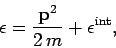
Consider a molecule of mass  in a gas which is sufficiently
dilute for the intermolecular forces to be negligible (i.e.,
an ideal gas).
The energy of the molecule is written
in a gas which is sufficiently
dilute for the intermolecular forces to be negligible (i.e.,
an ideal gas).
The energy of the molecule is written
 |
(533) |
where  is its momentum vector, and
 is its
internal (i.e., non-translational)
energy. The latter energy is due to molecular rotation, vibration, etc.
Translational degrees of freedom can be treated classically to an excellent
approximation, whereas internal degrees of freedom usually require a quantum
mechanical approach.
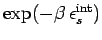
Classically, the probability of finding the molecule in a given internal
state with a position vector in the range
is its
internal (i.e., non-translational)
energy. The latter energy is due to molecular rotation, vibration, etc.
Translational degrees of freedom can be treated classically to an excellent
approximation, whereas internal degrees of freedom usually require a quantum
mechanical approach.
Classically, the probability of finding the molecule in a given internal
state with a position vector in the range  to
to
 ,
and a momentum vector in the range to
,
and a momentum vector in the range to
 , is proportional
to the number of cells (of ``volume''
, is proportional
to the number of cells (of ``volume''  ) contained in the corresponding region
of phase-space, weighted by the Boltzmann factor.
In fact, since classical phase-space is divided up into uniform cells,
the number of cells is just proportional to the ``volume'' of
the region under consideration. This ``volume'' is written
) contained in the corresponding region
of phase-space, weighted by the Boltzmann factor.
In fact, since classical phase-space is divided up into uniform cells,
the number of cells is just proportional to the ``volume'' of
the region under consideration. This ``volume'' is written
 .
Thus, the probability of finding the molecule in a given internal state
.
Thus, the probability of finding the molecule in a given internal state  is
is
 |
(534) |
where  is a probability density defined in the usual manner. The probability
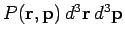 of finding the molecule in any internal state
with position and momentum vectors in the
specified range
is obtained by summing the above expression over all possible internal states.
The sum over
of finding the molecule in any internal state
with position and momentum vectors in the
specified range
is obtained by summing the above expression over all possible internal states.
The sum over
 just contributes a constant of
proportionality (since the internal states do not depend on
just contributes a constant of
proportionality (since the internal states do not depend on  or
or
 ), so
), so
 |
(535) |
Of course, we can multiply this probability by the total number of molecules
 in order
to obtain the mean number of molecules with position and momentum vectors in the
specified range.
in order
to obtain the mean number of molecules with position and momentum vectors in the
specified range.
Suppose that we now want to determine
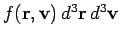 : i.e.,
the mean number of molecules with positions between and
, and velocities in the range
: i.e.,
the mean number of molecules with positions between and
, and velocities in the range  and
and
 .
Since
.
Since
 , it is easily seen that
 |
(536) |
where  is a constant of proportionality. This constant can be determined by
the condition
is a constant of proportionality. This constant can be determined by
the condition
 |
(537) |
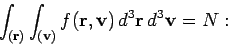
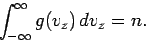
i.e., the sum over molecules with all possible positions and velocities gives
the total number of molecules, . The integral over the molecular position
coordinates just gives the volume  of the gas, since the Boltzmann factor
is independent of position. The integration over the velocity coordinates can
be reduced to the product of three identical integrals (one for
of the gas, since the Boltzmann factor
is independent of position. The integration over the velocity coordinates can
be reduced to the product of three identical integrals (one for  , one
for
, one
for  , and one for
  ), so we have
![\begin{displaymath}
C\, V \left[\int_{-\infty}^{\infty} \exp(-\beta\, m\,v_z^{~2}/2)\, dv_z\right]^3
= N.
\end{displaymath}](img1287.png) |
(538) |
Now,
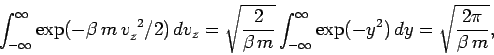 |
(539) |
so
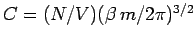 . Thus, the properly normalized distribution
function for molecular velocities is written
. Thus, the properly normalized distribution
function for molecular velocities is written
 |
(540) |
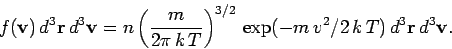
Here,  is the number density of the molecules. We
have omitted the variable in the argument of
is the number density of the molecules. We
have omitted the variable in the argument of  , since
clearly does not depend on position. In other words, the distribution of
molecular velocities is uniform in space. This is hardly surprising, since there
is nothing to distinguish one region of space from another in our calculation.
The above distribution is called the Maxwell velocity distribution,
because it was discovered by James Clark Maxwell in the middle of the nineteenth century.
The average number of molecules per unit volume with velocities in the
range to
is obviously
, since
clearly does not depend on position. In other words, the distribution of
molecular velocities is uniform in space. This is hardly surprising, since there
is nothing to distinguish one region of space from another in our calculation.
The above distribution is called the Maxwell velocity distribution,
because it was discovered by James Clark Maxwell in the middle of the nineteenth century.
The average number of molecules per unit volume with velocities in the
range to
is obviously
 .
.
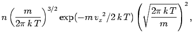
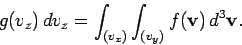
Let us consider the distribution of a given component of velocity: the  -component,
say. Suppose that
-component,
say. Suppose that  is the average number of molecules per unit volume
with the -component of velocity in the range to
is the average number of molecules per unit volume
with the -component of velocity in the range to  , irrespective
of the values of their other velocity components. It is fairly obvious that
this distribution is obtained from the Maxwell distribution by summing (integrating
actually) over all possible values of and , with in the specified
range. Thus,
, irrespective
of the values of their other velocity components. It is fairly obvious that
this distribution is obtained from the Maxwell distribution by summing (integrating
actually) over all possible values of and , with in the specified
range. Thus,
 |
(541) |
This gives
or
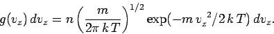 |
(543) |
Of course, this expression is properly normalized, so that
 |
(544) |
It is clear that each component (since there is nothing special about the -component) of the velocity is distributed with a Gaussian probability distribution
(see Sect. 2),
centred on a mean value
 |
(545) |
with variance
 |
(546) |
Equation (545) implies that each molecule is just as likely to be moving in the
plus -direction as in the minus -direction. Equation (546) can be rearranged
to give
 |
(547) |
in accordance with the equipartition theorem.
Note that Eq. (540) can be rewritten
![\begin{displaymath}
\frac{ f({\bf v}) \, d^3{\bf v}}{n} =\left[\frac{g(v_x)\,dv_...
...ac{g(v_y)\,dv_y}{n}\right]\left[\frac{g(v_z)\,dv_z}{n}\right],
\end{displaymath}](img1305.png) |
(548) |
where  and
and  are defined in an analogous way to
  .
Thus, the probability that the velocity lies in the range to
is just equal to the product of the probabilities
that the velocity components lie in their respective ranges.
In other words, the individual
velocity components act like statistically independent variables.
.
Thus, the probability that the velocity lies in the range to
is just equal to the product of the probabilities
that the velocity components lie in their respective ranges.
In other words, the individual
velocity components act like statistically independent variables.
Suppose that we now want to calculate  :
i.e., the average number of molecules
per unit volume with a speed
:
i.e., the average number of molecules
per unit volume with a speed  in the range
  to
to  . It is
obvious that we can obtain this quantity by adding up all molecules with speeds
in this range, irrespective of the direction of their velocities. Thus,
. It is
obvious that we can obtain this quantity by adding up all molecules with speeds
in this range, irrespective of the direction of their velocities. Thus,
 |
(549) |
where the integral extends over all velocities satisfying
 |
(550) |
This inequality is satisfied by a spherical shell of radius and thickness  in velocity space. Since
  only depends on
  ,
so
,
so
 , the above
integral is just
, the above
integral is just  multiplied by the volume of the spherical shell in
velocity space. So,
multiplied by the volume of the spherical shell in
velocity space. So,
 |
(551) |
which gives
 |
(552) |
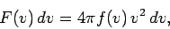
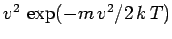
This is the famous Maxwell distribution of molecular speeds.
Of course, it is properly normalized, so that
 |
(553) |
Note that the Maxwell
distribution exhibits a maximum at some non-zero value of . The reason for
this is quite simple. As increases, the Boltzmann factor decreases,
but the volume of phase-space available to the molecule (which is
proportional to  ) increases: the net result is a distribution
with a non-zero maximum.
) increases: the net result is a distribution
with a non-zero maximum.
Figure 7:
The Maxwell velocity distribution as a function
of molecular speed in units of the most probable speed ( )
. Also shown are the
mean speed (
)
. Also shown are the
mean speed ( ) and the root mean square speed
(
) and the root mean square speed
( ).
).
 |
The mean molecular speed is given by
 |
(554) |
Thus, we obtain
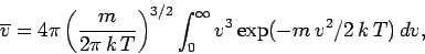 |
(555) |
or
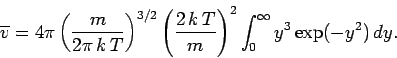 |
(556) |
Now
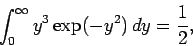 |
(557) |
so
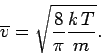 |
(558) |
A similar calculation gives
 |
(559) |
However, this result can also be obtained from the equipartition theorem.
Since
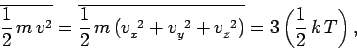 |
(560) |
then Eq. (559) follows immediately. It is easily demonstrated that the most probable
molecular speed (i.e., the maximum of the Maxwell distribution function) is
 |
(561) |
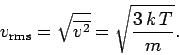
The speed of sound in an ideal gas is given by
 |
(562) |
where  is the ratio of specific heats. This can also be written
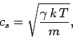 |
(563) |
since  and
and  . It is clear that the various average speeds which
we have just calculated are all of order the sound speed (i.e., a few hundred
meters per second at room temperature). In ordinary air (
. It is clear that the various average speeds which
we have just calculated are all of order the sound speed (i.e., a few hundred
meters per second at room temperature). In ordinary air ( ) the
sound speed is about 84% of the most probable molecular speed, and about
74% of the mean molecular speed. Since sound waves
ultimately propagate via molecular
motion, it makes sense that they travel at slightly less than the most probable
and mean
molecular speeds.
) the
sound speed is about 84% of the most probable molecular speed, and about
74% of the mean molecular speed. Since sound waves
ultimately propagate via molecular
motion, it makes sense that they travel at slightly less than the most probable
and mean
molecular speeds.
Figure 7 shows the Maxwell velocity distribution as a function
of molecular speed in units of the most probable speed. Also shown are the
mean speed and the root mean square speed.
It is difficult to directly verify the Maxwell velocity distribution. However, this
distribution can be verified indirectly by measuring the velocity distribution
of atoms exiting from a small hole in an oven. The velocity distribution of
the escaping atoms is closely related to, but slightly different from, the velocity
distribution inside the oven, since high velocity atoms escape more readily
than low velocity atoms. In fact, the predicted velocity distribution of
the escaping atoms varies like
 , in contrast
to the
, in contrast
to the
 variation of the velocity distribution
inside the oven. Figure 8 compares the measured and
theoretically predicted
velocity distributions of potassium atoms escaping from an oven at
variation of the velocity distribution
inside the oven. Figure 8 compares the measured and
theoretically predicted
velocity distributions of potassium atoms escaping from an oven at
 C. There is clearly very good agreement between the two.
Figure 8:
Comparison of the measured and theoretically
predicted velocity distributions of potassium atoms escaping from an oven at
C. Here, the measured transit time is directly proportional
to the atomic speed.
 |
Next: Quantum statistics
Up: Applications of statistical thermodynamics
Previous: Specific heats of solids
Richard Fitzpatrick
2006-02-02
![$\displaystyle n \left(\frac{m}{2\pi\, k\,T}\right)^{3/2}
\int_{(v_x)} \int_{(v_y)} \exp[- (m/2\, k\,T)(v_x^{~2}+v_y^{~2}+v_z^{~2})]\,
dv_x\,dv_y\, dv_z$](img1297.png)
![$\displaystyle n \left(\frac{m}{2\pi \,k\,T}\right)^{3/2} \exp(-m\,v_z^{~2}/ 2\,k\,T)
\left[\int_{-\infty}^{\infty} \exp(-m\,v_x^{~2}/ 2\,k\,T)\right]^2$](img1298.png)