


Next: The central limit theorem
Up: Probability theory
Previous: Application to the binomial
Consider a very large number of observations,  , made on a system
with two possible outcomes.
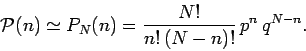
Suppose that the probability of outcome 1 is sufficiently large that
the average number of occurrences after
, made on a system
with two possible outcomes.
Suppose that the probability of outcome 1 is sufficiently large that
the average number of occurrences after  observations is much greater than unity:
 |
(54) |
In this limit, the standard deviation of  is also much greater than unity,
 |
(55) |
implying that there are very many probable values of scattered about the
mean value
 .
This suggests that the probability of obtaining occurrences
of outcome 1
does not change significantly in going from one possible value of
to an adjacent value:
.
This suggests that the probability of obtaining occurrences
of outcome 1
does not change significantly in going from one possible value of
to an adjacent value:
 |
(56) |
In this situation, it is useful to regard the probability as a smooth
function of . Let  be a continuous variable which is
interpreted as the number of occurrences of outcome 1 (after
observations) whenever it takes
on a positive integer value. The probability that lies between
and
be a continuous variable which is
interpreted as the number of occurrences of outcome 1 (after
observations) whenever it takes
on a positive integer value. The probability that lies between
and  is defined
 |
(57) |
where  is called the probability density, and is independent
of
is called the probability density, and is independent
of  . The probability can be written in this form because
 can always be expanded as a Taylor series in , and must go
to zero as
can always be expanded as a Taylor series in , and must go
to zero as
 .
We can write
.
We can write
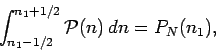 |
(58) |
which is equivalent to smearing out the discrete probability  over the range
  . Given Eq. (56), the above relation
can be approximated
. Given Eq. (56), the above relation
can be approximated
 |
(59) |
For large , the relative width of the probability distribution function
is small:
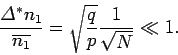 |
(60) |
This suggests that is strongly peaked around the mean value
 . Suppose that
 attains
its maximum value at
attains
its maximum value at  (where we expect
 ). Let us Taylor expand
  around .
Note that we expand the slowly varying function
,
instead of the rapidly varying function ,
because the Taylor expansion of
does not converge sufficiently rapidly in the
vicinity of to be useful.
We can write
around .
Note that we expand the slowly varying function
,
instead of the rapidly varying function ,
because the Taylor expansion of
does not converge sufficiently rapidly in the
vicinity of to be useful.
We can write
 |
(61) |
where
 |
(62) |
By definition,
if corresponds to the maximum
value of
.
It follows from Eq. (59) that
 |
(65) |
If is a large integer, such that  , then
  is almost a
continuous function of , since changes by only a relatively
small amount when is incremented by unity.
Hence,
is almost a
continuous function of , since changes by only a relatively
small amount when is incremented by unity.
Hence,
![\begin{displaymath}
\frac{d\ln n!}{dn} \simeq \frac{\ln\,(n+1)!-\ln n!}{1} =
\ln\!\left[\frac{(n+1)!}{n!}\right] = \ln\,(n+1),
\end{displaymath}](img194.png) |
(66) |
giving
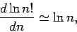 |
(67) |
for . The integral of this relation
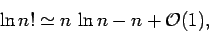 |
(68) |
valid for , is called Stirling's approximation, after the Scottish
mathematician James Stirling who first obtained it in 1730.
According to Eq. (65),
 |
(69) |
Hence, if  then
then
 |
(70) |
giving
 |
(71) |
since  . Thus, the maximum of
occurs exactly
at the mean value of , which equals
.
. Thus, the maximum of
occurs exactly
at the mean value of , which equals
.
Further differentiation of Eq. (65) yields
 |
(72) |
since . Note that  , as required. The above relation
can also be written
, as required. The above relation
can also be written
 |
(73) |
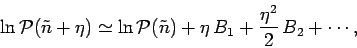
It follows from the above that the Taylor expansion of can be written
 |
(74) |
Taking the exponential of both sides yields
![\begin{displaymath}
{\cal P}(n)\simeq {\cal P}(\overline{n_1})\exp\!\left[-
\frac{(n-\overline{n_1})^2}{2\,({\mit\Delta}^\ast n_1)^2}\right].
\end{displaymath}](img205.png) |
(75) |
The constant
 is most conveniently
fixed by making use
of the normalization condition
is most conveniently
fixed by making use
of the normalization condition
 |
(76) |
which translates to
 |
(77) |
for a continuous distribution function. Since we only expect
to be significant when
lies in the relatively narrow range
 , the limits of integration in the above
expression can be replaced by
, the limits of integration in the above
expression can be replaced by  with negligible error.
Thus,
with negligible error.
Thus,
 |
(78) |
As is well-known,
 |
(79) |
so it follows from the normalization condition (78) that
 |
(80) |
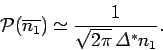
Finally, we obtain
![\begin{displaymath}
{\cal P}(n) \simeq \frac{1}{\sqrt{2\pi} \,{\mit\Delta}^\ast ...
...ac{(n-\overline{n_1})^2}{2\,({\mit\Delta}^\ast n_1)^2}\right].
\end{displaymath}](img214.png) |
(81) |
This is the famous Gaussian distribution function, named after the
German mathematician Carl Friedrich Gauss, who discovered it whilst
investigating the distribution of errors in measurements. The Gaussian
distribution is only valid in the limits and
 .
.
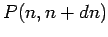
Suppose we were to
plot the probability
against the integer variable , and then
fit a continuous curve through the discrete points thus obtained. This curve
would be
equivalent to the continuous probability density curve , where
is the continuous version of . According to Eq. (81), the
probability density attains its maximum
value when equals the mean
of , and
is also symmetric about this point. In fact, when plotted with the
appropriate ratio of vertical to horizontal scalings, the Gaussian probability
density curve looks rather like the outline of a
bell centred on
 . Hence, this curve is sometimes
called a bell curve.
At one standard deviation away from the mean value, i.e.,
. Hence, this curve is sometimes
called a bell curve.
At one standard deviation away from the mean value, i.e.,
 , the probability density is
about 61% of its peak value. At two standard deviations away from the mean
value, the probability density is about 13.5% of its peak value.
Finally,
at three standard deviations away from the mean value, the probability
density is only about 1% of its peak value. We conclude
that there is
very little chance indeed that lies more than about three standard deviations
away from its mean value. In other words, is almost certain to lie in the
relatively narrow range
, the probability density is
about 61% of its peak value. At two standard deviations away from the mean
value, the probability density is about 13.5% of its peak value.
Finally,
at three standard deviations away from the mean value, the probability
density is only about 1% of its peak value. We conclude
that there is
very little chance indeed that lies more than about three standard deviations
away from its mean value. In other words, is almost certain to lie in the
relatively narrow range
 . This is a very well-known result.
In the above analysis, we have gone from a discrete probability
function to a continuous probability density .
The normalization condition becomes
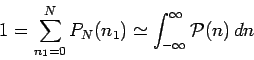 |
(82) |
under this transformation. Likewise, the evaluations of the mean and
variance of the distribution are written
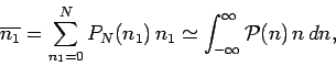 |
(83) |
and
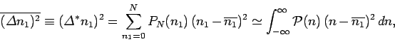 |
(84) |
respectively. These results
follow as simple generalizations of previously established results for
the discrete function .
The limits of integration in the above expressions
can be approximated as because is only
non-negligible in a relatively narrow range of .
Finally, it is easily demonstrated that Eqs. (82)-(84) are indeed
true by substituting in the Gaussian probability density,
Eq. (81), and then performing a few elementary integrals.
Next: The central limit theorem
Up: Probability theory
Previous: Application to the binomial
Richard Fitzpatrick
2006-02-02