Specific Heats

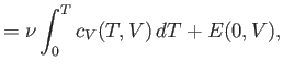
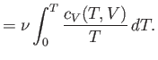
We have discussed the internal energies and entropies of substances (mostly ideal gases) at some length. Unfortunately, these quantities cannot be directly measured. Instead, they must be inferred from other information. The thermodynamic property of substances that is the easiest to measure is, of course, the heat capacity, or specific heat. In fact, once the variation of the specific heat with temperature is known, both the internal energy and entropy can be easily reconstructed via

$$E (T, V) = \nu \int_0^T c_V(T, V) dT + E(0,V),$$ (7.156)

$$S(T, V) = \nu \int_0^T \frac{c_V(T,V)}{T} dT.$$ (7.157)

Here, use has been made of $dS = {\mathchar'26\mkern-11mud}Q/T$ , and the third law of thermodynamics. Clearly, the optimum way of verifying the results of statistical thermodynamics is to compare the theoretically predicted heat capacities with the experimentally measured values.

Classical physics, in the guise of the equipartition theorem, says that each independent degree of freedom associated with a quadratic term in the energy possesses an average energy $(1/2) k T$ in thermal equilibrium at temperature $T$ . Consider a substance made up of $N$ molecules. Every molecular degree of freedom contributes $(1/2) N k T$ , or $(1/2) \nu R T$ , to the mean energy of the substance (with the tacit proviso that each degree of freedom is associated with a quadratic term in the energy). Thus, the contribution to the molar heat capacity at constant volume (we wish to avoid the complications associated with any external work done on the substance) is

$$\frac{1}{\nu}\left( \frac{\partial \overline{E}}{\partial T}\righ... ...rac{1}{\nu} \frac{\partial[ (1/2) \nu R T] }{\partial T}= \frac{1}{2} R,$$ (7.158)

per molecular degree of freedom. The total classical heat capacity is therefore

$$c_V = \frac{g}{2} R,$$ (7.159)

where $g$ is the number of molecular degrees of freedom. Because large complicated molecules clearly have very many more degrees of freedom than small simple molecules, the previous formula predicts that the molar heat capacities of substances made up of the former type of molecules should greatly exceed those of substances made up of the latter. In fact, the experimental heat capacities of substances containing complicated molecules are generally greater than those of substances containing simple molecules, but by nowhere near the large factor predicted in Equation (7.159). This equation also implies that heat capacities are temperature independent. In fact, this is not the case for most substances. Experimental heat capacities generally increase with increasing temperature. These two experimental facts pose severe problems for classical physics. Incidentally, these problems were fully appreciated as far back as 1850. Stories that physicists at the end of the nineteenth century thought that classical physics explained absolutely everything are largely apocryphal.

The equipartition theorem (and the whole classical approximation) is only valid when the typical thermal energy, $k T$ , greatly exceeds the spacing between quantum energy levels. Suppose that the temperature is sufficiently low that this condition is not satisfied for one particular molecular degree of freedom. In fact, suppose that $k T$ is much less than the spacing between the energy levels. According to Section 7.11, in this situation, the degree of freedom only contributes the ground-state energy, $E_0$ (say) to the mean energy of the molecule. Now, the ground-state energy can be a quite complicated function of the internal properties of the molecule, but is certainly not a function of the temperature, because this is a collective property of all molecules. It follows that the contribution to the molar heat capacity is

$$\frac{1}{\nu}\left( \frac{\partial [N E_0]}{\partial T}\right)_V = 0.$$ (7.160)

Thus, if $k T$ is much less than the spacing between the energy levels then the degree of freedom contributes nothing at all to the molar heat capacity. We say that this particular degree of freedom is ``frozen out.'' Clearly, at very low temperatures, just about all degrees of freedom are frozen out. As the temperature is gradually increased, degrees of freedom successively kick in, and eventually contribute their full $(1/2) R$ to the molar heat capacity, as $k T$ approaches, and then greatly exceeds, the spacing between their quantum energy levels. We can use these simple ideas to explain the behaviors of most experimental heat capacities.

To make further progress, we need to estimate the typical spacing between the quantum energy levels associated with various degrees of freedom. We can do this by observing the frequency of the electromagnetic radiation emitted and absorbed during transitions between these energy levels. If the typical spacing between energy levels is ${\mit\Delta} E$ then transitions between the various levels are associated with photons of frequency $\nu$ , where $h \nu = {\mit\Delta} E$ . (Here, $h$ is Planck's constant.) We can define an effective temperature of the radiation via $h \nu = k T_{\rm rad}$ . If $T\gg T_{\rm rad}$ then $k T \gg {\mit\Delta} E$ , and the degree of freedom makes its full contribution to the heat capacity. On the other hand, if $T\ll T_{\rm rad}$ then $k T \ll {\mit\Delta} E$ , and the degree of freedom is frozen out. Table 7.1 lists the ``temperatures'' of various different types of radiation. It is clear that degrees of freedom that give rise to emission or absorption of radio or microwave radiation contribute their full $(1/2) R$ to the molar heat capacity at room temperature. On the other hand, degrees of freedom that give rise to emission or absorption in the visible, ultraviolet, X-ray, or $\gamma$ -ray regions of the electromagnetic spectrum are frozen out at room temperature. Degrees of freedom that emit or absorb infrared radiation are on the border line.

Table 7.1: Effective ``temperatures'' of various types of electromagnetic radiation.

Radiation type	Frequency (hz)	$T_{\rm rad}$ (K)
Radio	$<10^{ 9}$	$<0.05$
Microwave	$10^{ 9}$ - $10^{ 11}$	$0.05$ - $5$
Infrared	$10^{ 11}$ - $10^{ 14}$	$5$ - $5000$
Visible	$5 \times 10^{ 14}$	$2\times 10^{ 4}$
Ultraviolet	$10^{ 15}$ - $10^{ 17}$	$5\times 10^{ 4}$ - $5\times 10^{ 6}$
X-ray	$10^{ 17}$ - $10^{ 20}$	$5\times 10^{ 6}$ - $5\times 10^{ 9}$
$\gamma$ -ray	$>10^{ 20}$	$>5\times 10^{ 9}$