Next: Generalized Momenta
Up: Classical Mechanics
Previous: Generalized Forces
The Cartesian equations of motion of our dynamical system take
the form
 |
(B.9) |
for
 , where
 are each equal to the mass of the
first particle,
are each equal to the mass of the
first particle,
 are each equal to the mass of the
second particle, et cetera. Furthermore, the kinetic energy of the
system can be written
are each equal to the mass of the
second particle, et cetera. Furthermore, the kinetic energy of the
system can be written
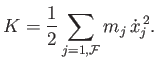 |
(B.10) |
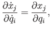
Now, because
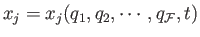 , we can write
 |
(B.11) |
for
.
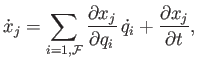
Hence, it follows that
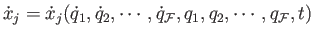 . According to the
previous equation,
. According to the
previous equation,
 |
(B.12) |
where we are treating the  and the
  as independent
variables.
as independent
variables.
Multiplying Equation (B.12) by  , and then differentiating
with respect to time, we obtain
, and then differentiating
with respect to time, we obtain
 |
(B.13) |
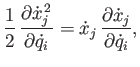
Now,
 |
(B.14) |
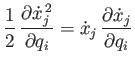
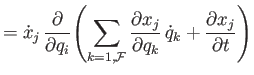
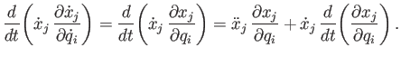
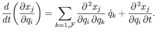
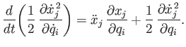
Furthermore,
 |
(B.15) |
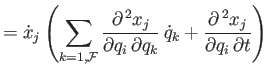
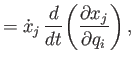
and
where use has been made of Equation (B.14). Thus, it follows
from Equations (B.13), (B.15), and (B.16) that
 |
(B.17) |
Let us take the previous equation, multiply by  , and then sum over all
  .
We obtain
.
We obtain
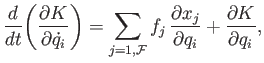 |
(B.18) |
where use has been made of Equations (B.9) and (B.10). Thus, it follows from Equation (B.6) that
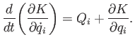 |
(B.19) |
Finally, making use of Equation (B.8), we get
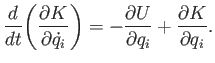 |
(B.20) |
It is helpful to introduce a function  , called the Lagrangian, which
is defined as the difference between the kinetic and potential energies of the dynamical system under investigation:
, called the Lagrangian, which
is defined as the difference between the kinetic and potential energies of the dynamical system under investigation:
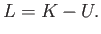 |
(B.21) |
Because the potential energy,  , is clearly independent of the
, it follows from Equation (B.20) that
, is clearly independent of the
, it follows from Equation (B.20) that
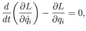 |
(B.22) |
for
 . This equation is known as Lagrange's equation.
According to the previous analysis, if we can express the kinetic and
potential energies of our dynamical system solely in terms of our generalized
coordinates, and their time derivatives, then we can immediately write
down the equations of motion of the system, expressed in terms
of the generalized coordinates, using Lagrange's equation, (B.22).
Unfortunately, this scheme only works for energy-conserving systems.
Next: Generalized Momenta
Up: Classical Mechanics
Previous: Generalized Forces
Richard Fitzpatrick
2016-01-25