Harmonic Perturbations

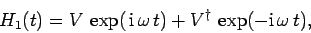
Consider a (Hermitian) perturbation which oscillates sinusoidally in time. This is usually termed a harmonic perturbation. Such a perturbation takes the form

$$H_1(t) = V \exp( {\rm i} \omega t) + V^\dag \exp(-{\rm i} \omega t),$$ (1067)

where $V$ is, in general, a function of position, momentum, and spin operators.

It follows from Eqs. (1064) and (1067) that, to first-order,

$$c_f(t) = - \frac{\rm i}{\hbar}\int_0^t\left[V_{fi} \exp( {... ... i} \omega t')\right] \exp( {\rm i} \omega_{fi} t') dt',$$ (1068)

where

$$V_{fi} = \langle f\vert V\vert i\rangle,$$ (1069)

$$V_{fi}^\dag = \langle f\vert V^\dag \vert i\rangle = \langle i\vert V\vert f\rangle^\ast.$$ (1070)

Integration with respect to $t'$ yields

$$c_f(t) = - \frac{{\rm i} t}{\hbar}\left(V_{fi} \exp\left[ {\rm i} (\om... ...\omega_{fi}) t/2\right]{\rm sinc}\left[(\omega+\omega_{fi}) t/2\right]\right.$$

$$\left.+V_{fi}^\dag \exp\left[-{\rm i} (\omega-\omega_{fi}) t/2\right]{\rm sinc}\left[(\omega-\omega_{fi}) t/2\right]\right),$$ (1071)

where

$${\rm sinc} x\equiv \frac{\sin x}{x}.$$ (1072)

Figure 25: The functions ${\rm sinc}(x)$ (dashed curve) and ${\rm sinc}^2(x)$ (solid curve). The vertical dotted lines denote the region $\vert x\vert\leq \pi$.

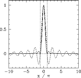Now, the function ${\rm sinc}(x)$ takes its largest values when $\vert x\vert\stackrel {_{\normalsize <}}{_{\normalsize\sim}}\pi$, and is fairly negligible when $\vert x\vert\gg \pi$ (see Fig. 25). Thus, the first and second terms on the right-hand side of Eq. (1071) are only non-negligible when

$$\vert\omega+\omega_{fi}\vert\stackrel {_{\normalsize <}}{_{\normalsize\sim}}\frac{2\pi}{t},$$ (1073)

and

$$\vert\omega-\omega_{fi}\vert\stackrel {_{\normalsize <}}{_{\normalsize\sim}}\frac{2\pi}{t},$$ (1074)

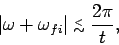
respectively. Clearly, as $t$ increases, the ranges in $\omega$ over which these two terms are non-negligible gradually shrink in size. Eventually, when $t\gg 2\pi/\vert\omega_{fi}\vert$, these two ranges become strongly non-overlapping. Hence, in this limit, $P_{i\rightarrow f}=\vert c_f\vert^2$ yields

$$P_{i\rightarrow f}(t) = \frac{t^2}{\hbar^2}\left\{ \vert V_{... ...} {\rm sinc}^2\left[(\omega-\omega_{fi}) t/2\right]\right\}.$$ (1075)

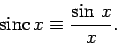
Now, the function ${\rm sinc}^2(x)$ is very strongly peaked at $x=0$, and is completely negligible for $\vert x\vert\stackrel {_{\normalsize >}}{_{\normalsize\sim}}\pi$ (see Fig. 25). It follows that the above expression exhibits a resonant response to the applied perturbation at the frequencies $\omega=\pm\omega_{fi}$. Moreover, the widths of these resonances decease linearly as time increases. At each of the resonances (i.e., at $\omega=\pm\omega_{fi}$), the transition probability $P_{i\rightarrow f}(t)$ varies as $t^2$ [since ${\rm sinh} (0)=1$]. This behaviour is entirely consistent with our earlier result (1044), for the two-state system, in the limit $\gamma t\ll 1$ (recall that our perturbative solution is only valid as long as $P_{i\rightarrow f}\ll 1$).

The resonance at $\omega=-\omega_{fi}$ corresponds to

$$E_f - E_i = -\hbar \omega.$$ (1076)

This implies that the system loses energy $\hbar \omega$ to the perturbing field, whilst making a transition to a final state whose energy is less than the initial state by $\hbar \omega$. This process is known as stimulated emission. The resonance at $\omega=\omega_{fi}$ corresponds to

$$E_f - E_i = \hbar \omega.$$ (1077)

This implies that the system gains energy $\hbar \omega$ from the perturbing field, whilst making a transition to a final state whose energy is greater than that of the initial state by $\hbar \omega$. This process is known as absorption.

Stimulated emission and absorption are mutually exclusive processes, since the first requires $\omega_{fi}<0$, whereas the second requires $\omega_{fi}>0$. Hence, we can write the transition probabilities for both processes separately. Thus, from (1075), the transition probability for stimulated emission is

$$P_{i\rightarrow f}^{stm}(t) = \frac{t^2}{\hbar^2} \vert V_... ...ert^{ 2} {\rm sinc}^2\left[(\omega-\omega_{if}) t/2\right],$$ (1078)

where we have made use of the facts that $\omega_{if}=-\omega_{fi}>0$, and $\vert V_{fi}\vert^2=\vert V_{if}^\dag \vert^2$. Likewise, the transition probability for absorption is

$$P_{i\rightarrow f}^{abs}(t) = \frac{t^2}{\hbar^2} \vert V_... ...ert^{ 2} {\rm sinc}^2\left[(\omega-\omega_{fi}) t/2\right].$$ (1079)