Simple Harmonic Oscillator

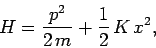
The classical Hamiltonian of a simple harmonic oscillator is

$$H = \frac{p^2}{2 m} + \frac{1}{2} K x^2,$$ (389)

where $K>0$ is the so-called force constant of the oscillator. Assuming that the quantum mechanical Hamiltonian has the same form as the classical Hamiltonian, the time-independent Schrödinger equation for a particle of mass $m$ and energy $E$ moving in a simple harmonic potential becomes

$$\frac{d^2\psi}{dx^2} = \frac{2 m}{\hbar^2}\left(\frac{1}{2} K x^2-E\right)\psi.$$ (390)

Let $\omega = \sqrt{K/m}$, where $\omega$ is the oscillator's classical angular frequency of oscillation. Furthermore, let

$$y = \sqrt{\frac{m \omega}{\hbar}} x,$$ (391)

and

$$\epsilon = \frac{2 E}{\hbar \omega}.$$ (392)

Equation (390) reduces to

$$\frac{d^2\psi}{dy^2} - (y^2-\epsilon) \psi = 0.$$ (393)

We need to find solutions to the above equation which are bounded at infinity: i.e., solutions which satisfy the boundary condition $\psi\rightarrow 0$ as $\vert y\vert\rightarrow\infty$.

Consider the behavior of the solution to Eq. (393) in the limit $\vert y\vert\gg 1$. As is easily seen, in this limit the equation simplifies somewhat to give

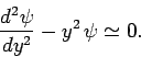$$\frac{d^2\psi}{dy^2} - y^2 \psi \simeq 0.$$ (394)

The approximate solutions to the above equation are

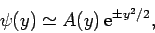$$\psi(y) \simeq A(y) {\rm e}^{\pm y^2/2},$$ (395)

where $A(y)$ is a relatively slowly varying function of $y$. Clearly, if $\psi(y)$ is to remain bounded as $\vert y\vert\rightarrow\infty$ then we must chose the exponentially decaying solution. This suggests that we should write

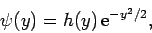$$\psi(y) = h(y) {\rm e}^{-y^2/2},$$ (396)

where we would expect $h(y)$ to be an algebraic, rather than an exponential, function of $y$.

Substituting Eq. (396) into Eq. (393), we obtain

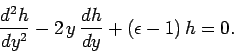$$\frac{d^2h}{dy^2} - 2 y \frac{dh}{dy} + (\epsilon-1) h = 0.$$ (397)

Let us attempt a power-law solution of the form

$$h(y) = \sum_{i=0}^\infty c_i y^i.$$ (398)

Inserting this test solution into Eq. (397), and equating the coefficients of $y^i$, we obtain the recursion relation

$$c_{i+2} = \frac{(2 i-\epsilon+1)}{(i+1) (i+2)} c_i.$$ (399)

Consider the behavior of $h(y)$ in the limit $\vert y\vert\rightarrow\infty$. The above recursion relation simplifies to

$$c_{i+2} \simeq \frac{2}{i} c_i.$$ (400)

Hence, at large $\vert y\vert$, when the higher powers of $y$ dominate, we have

$$h(y) \sim C \sum_{j}\frac{y^{2 j}}{j!}\sim C {\rm e}^{ y^2}.$$ (401)

It follows that $\psi(y) = h(y) \exp(-y^2/2)$ varies as $\exp( y^2/2)$ as $\vert y\vert\rightarrow\infty$. This behavior is unacceptable, since it does not satisfy the boundary condition $\psi\rightarrow 0$ as $\vert y\vert\rightarrow\infty$. The only way in which we can prevent $\psi$ from blowing up as $\vert y\vert\rightarrow\infty$ is to demand that the power series (398) terminate at some finite value of $i$. This implies, from the recursion relation (399), that

$$\epsilon = 2 n+1,$$ (402)

where $n$ is a non-negative integer. Note that the number of terms in the power series (398) is $n+1$. Finally, using Eq. (392), we obtain

$$E = (n+1/2) \hbar \omega,$$ (403)

for $n=0,1,2,\cdots$.

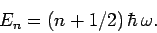
Hence, we conclude that a particle moving in a harmonic potential has quantized energy levels which are equally spaced. The spacing between successive energy levels is $\hbar \omega$, where $\omega$ is the classical oscillation frequency. Furthermore, the lowest energy state ($n=0$) possesses the finite energy $(1/2) \hbar \omega$. This is sometimes called zero-point energy. It is easily demonstrated that the (normalized) wavefunction of the lowest energy state takes the form

$$\psi_0(x) = \frac{{\rm e}^{-x^2/2 d^2}}{\pi^{1/4} \sqrt{d}},$$ (404)

where $d=\sqrt{\hbar/m \omega}$.

Let $\psi_n(x)$ be an energy eigenstate of the harmonic oscillator corresponding to the eigenvalue

$$E_n = (n+1/2) \hbar \omega.$$ (405)

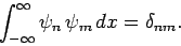
Assuming that the $\psi_n$ are properly normalized (and real), we have

$$\int_{-\infty}^\infty \psi_n \psi_m dx = \delta_{nm}.$$ (406)

Now, Eq. (393) can be written

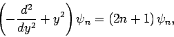$$\left(-\frac{d^2}{d y^2}+y^2\right)\psi_n = (2n+1) \psi_n,$$ (407)

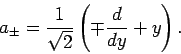
where $x = d y$, and $d=\sqrt{\hbar/m \omega}$. It is helpful to define the operators

$$a_\pm = \frac{1}{\sqrt{2}}\left(\mp \frac{d}{dy}+y\right).$$ (408)

As is easily demonstrated, these operators satisfy the commutation relation

$$[a_+,a_-]= -1.$$ (409)

Using these operators, Eq. (407) can also be written in the forms

$$a_+ a_- \psi_n = n \psi_n,$$ (410)

or

$$a_- a_+ \psi_n = (n+1) \psi_n.$$ (411)

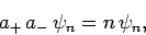
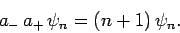
The above two equations imply that

$$a_+ \psi_n = \sqrt{n+1} \psi_{n+1},$$ (412)

$$a_- \psi_n = \sqrt{n} \psi_{n-1}.$$ (413)

We conclude that $a_+$ and $a_-$ are raising and lowering operators, respectively, for the harmonic oscillator: i.e., operating on the wavefunction with $a_+$ causes the quantum number $n$ to increase by unity, and vice versa. The Hamiltonian for the harmonic oscillator can be written in the form

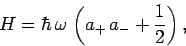$$H = \hbar \omega \left(a_+ a_- + \frac{1}{2}\right),$$ (414)

from which the result

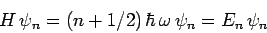$$H \psi_n = (n+1/2) \hbar \omega \psi_n = E_n \psi_n$$ (415)

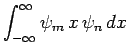
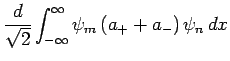
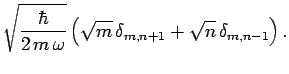
is readily deduced. Finally, Eqs. (406), (412), and (413) yield the useful expression

$$\int_{-\infty}^\infty \psi_m x \psi_n dx = \frac{d}{\sqrt{2}}\int_{-\infty}^{\infty}\psi_m (a_+ + a_-) \psi_n dx$$ (416)

$$= \sqrt{\frac{\hbar}{2 m \omega}}\left(\sqrt{m} \delta_{m,n+1} + \sqrt{n} \delta_{m,n-1}\right).$$