Next: Helium Atom
Up: Variational Methods
Previous: Introduction
Suppose that we wish to solve the time-independent Schrödinger equation
 |
(1167) |
where  is a known (presumably complicated) time-independent Hamiltonian. Let
  be a normalized trial solution to the above equation.
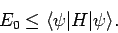
The variational principle states, quite simply, that the
ground-state energy,
be a normalized trial solution to the above equation.
The variational principle states, quite simply, that the
ground-state energy,  , is always less than or equal to the expectation
value of calculated with the trial wavefunction: i.e.,
, is always less than or equal to the expectation
value of calculated with the trial wavefunction: i.e.,
 |
(1168) |
Thus, by varying until the expectation value of is minimized, we can
obtain an approximation to the wavefunction and energy of the ground-state.
Let us prove the variational principle.
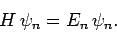
Suppose that the  and the
  are the true eigenstates and eigenvalues
of : i.e.,
are the true eigenstates and eigenvalues
of : i.e.,
 |
(1169) |
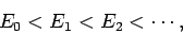
Furthermore, let
 |
(1170) |
so that  is the ground-state,
  the first excited state,
etc. The are assumed to be orthonormal:
i.e.,
the first excited state,
etc. The are assumed to be orthonormal:
i.e.,
 |
(1171) |
If our trial wavefunction is properly normalized then
we can write
 |
(1172) |
where
 |
(1173) |
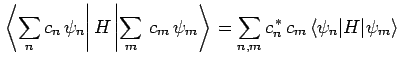
Now, the expectation value of , calculated with , takes the
form
where use has been made of Eqs. (1169) and (1171).
So, we can write
 |
(1175) |
However, Eq. (1173) can be rearranged to give
 |
(1176) |
Combining the previous two equations, we obtain
 |
(1177) |
Now, the second term on the right-hand side of the above expression
is positive definite, since  for all
  [see (1170)].
Hence, we obtain the desired result
[see (1170)].
Hence, we obtain the desired result
 |
(1178) |
Suppose that we have found a good approximation,
 , to the ground-state
wavefunction. If is a normalized trial wavefunction which is
orthogonal to
(i.e.,
, to the ground-state
wavefunction. If is a normalized trial wavefunction which is
orthogonal to
(i.e.,
 )
then, by repeating the above analysis, we can easily demonstrate that
)
then, by repeating the above analysis, we can easily demonstrate that
 |
(1179) |
Thus, by varying until the expectation value of is minimized, we can
obtain an approximation to the wavefunction and energy of the first excited state. Obviously, we can continue this process until we have approximations
to all of the stationary eigenstates. Note, however, that the errors are clearly cumulative in this method,
so that any approximations to highly excited states are unlikely to be very accurate. For this reason, the variational method is generally only
used to calculate the ground-state and first few excited states of
complicated quantum systems.
Next: Helium Atom
Up: Variational Methods
Previous: Introduction
Richard Fitzpatrick
2010-07-20