Next: Cutoffs Up: Waves in Inhomogeneous Plasmas Previous: Introduction Contents
 , propagating along the
  -axis in an unmagnetized plasma
whose refractive index,
-axis in an unmagnetized plasma
whose refractive index,  , is a function of . Let us assume that
the wave normal is initially aligned along the -axis, and, furthermore, that
the wave starts off polarized in the
, is a function of . Let us assume that
the wave normal is initially aligned along the -axis, and, furthermore, that
the wave starts off polarized in the  -direction. It is
easily demonstrated that the wave normal subsequently remains aligned along
the -axis, and also that the polarization
state does not change.
Thus, the wave is fully described by
-direction. It is
easily demonstrated that the wave normal subsequently remains aligned along
the -axis, and also that the polarization
state does not change.
Thus, the wave is fully described by
 |
(6.1) |
 |
(6.2) |
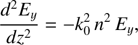
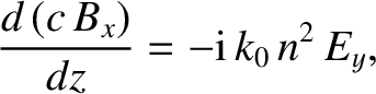
 and
and  satisfy
the differential equations
and
respectively. Here,
satisfy
the differential equations
and
respectively. Here,
 is the wavenumber
in free space. Of course, the actual wavenumber is
is the wavenumber
in free space. Of course, the actual wavenumber is  .
.
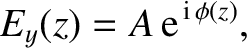
The solution of Equation (6.3) for the case of a homogeneous plasma, for which
is constant, is simply
 is a constant, and
The solution (6.5)
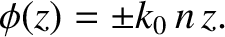
represents a wave of constant amplitude , and phase
is a constant, and
The solution (6.5)
represents a wave of constant amplitude , and phase  . According to
Equation (6.6),
there are two independent waves that can propagate through the plasma.
The upper sign corresponds to a wave that propagates in the
. According to
Equation (6.6),
there are two independent waves that can propagate through the plasma.
The upper sign corresponds to a wave that propagates in the  -direction,
whereas the lower sign corresponds to a wave that propagates in the
-direction,
whereas the lower sign corresponds to a wave that propagates in the
 -direction. Both waves propagate at the constant phase-velocity
  .
.
In general, if  then the solution of Equation (6.3) does not remotely resemble
the wave-like solution (6.5). However, in the limit in which
then the solution of Equation (6.3) does not remotely resemble
the wave-like solution (6.5). However, in the limit in which  is
a “slowly varying” function of (exactly how slowly varying is something that
will be established later on), we expect to recover wave-like solutions.
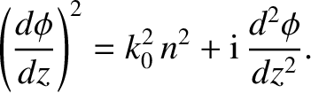
Let us suppose that is indeed a “slowly varying” function, and let us try
substituting the wave-like solution (6.5) into Equation (6.3). We obtain
is
a “slowly varying” function of (exactly how slowly varying is something that
will be established later on), we expect to recover wave-like solutions.
Let us suppose that is indeed a “slowly varying” function, and let us try
substituting the wave-like solution (6.5) into Equation (6.3). We obtain
is a constant then
 .
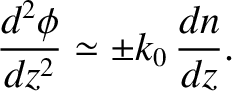
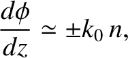
It is, therefore, reasonable to suppose that if is a “slowly varying” function
then the last term on the right-hand side of the previous equation is relatively small. Thus, to a first approximation, Equation (6.7) yields
.
It is, therefore, reasonable to suppose that if is a “slowly varying” function
then the last term on the right-hand side of the previous equation is relatively small. Thus, to a first approximation, Equation (6.7) yields
 |
(6.8) |
can
be regarded as a “slowly varying” function of [i.e., the second term on the right-hand side of Equation (6.7) is
negligible compared to the first] as long as
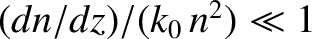 .
In other words, the approximation holds provided that the variation
lengthscale of the refractive index is far longer than the wavelength of the wave.
.
In other words, the approximation holds provided that the variation
lengthscale of the refractive index is far longer than the wavelength of the wave.
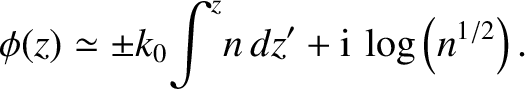
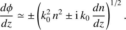
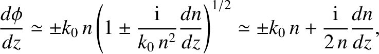
The second approximation to the solution is obtained by substituting Equation (6.9) into the right-hand side of Equation (6.7):
 |
(6.10) |
 |
(6.11) |
 |
(6.14) |
We can test to what extent expression (6.13) is a good solution of Equation (6.3) by substituting this expression into the left-hand side of the equation. The result is
![$\displaystyle \frac{1}{n^{1/2}}\left[ \frac{3}{4}\left(\frac{1}{n}
\frac{dn}{dz...
...\frac{1}{n}
\frac{dn}{dz}\right)^2 -\frac{1}{2\,n}\frac{d^2 n}{dz^2}\right]E_y.$](img1937.png) |
||
| (6.15) |
 . Hence, the
condition for Equation (6.13) to be a good solution of Equation (6.3)
becomes
. Hence, the
condition for Equation (6.13) to be a good solution of Equation (6.3)
becomes
The solutions
to the non-uniform wave equations (6.3) and (6.4) are usually referred to as WKB solutions, in honor of G. Wentzel (Wentzel 1926), H.A. Kramers (Kramers 1926), and L. Brillouin (Brilloiun 1926), who are credited with independently discovering these solutions (in a quantum mechanical context) in 1926. Actually, H. Jeffries (Jeffries 1924) wrote a paper on WKB solutions (in a wave propagation context) in 1924. Hence, these solutions are sometimes called the WKBJ solutions (or even the JWKB solutions). To be strictly accurate, the WKB solutions were first discussed by Liouville (Liouville 1837) and Green (Green 1837) in 1837, and again by Rayleigh (Rayleigh 1912) in 1912. In the following, we refer to Equations (6.17) and (6.18) as WKB solutions, because this is what they are most commonly called. However, it should be understood that, in doing so, we are not making any definitive statement as to the credit due to various scientists in discovering them. More information about WKB solutions can be found in the classic monograph of Heading (Heading 1962).
If a propagating wave is normally incident on an interface
at which the
refractive index suddenly changes (for instance, if a light
wave propagating through
air is normally incident on a glass slab) then there is generally
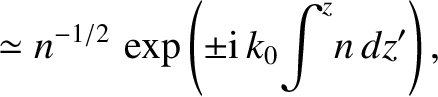
significant reflection of the wave (Fitzpatrick 2013). However, according to the WKB solutions,
(6.17) and (6.18), when a propagating wave is normally incident on a medium in which
the refractive index changes slowly along the direction of propagation of the
wave then the wave is not reflected at all. This is true
even if the refractive index
varies very substantially along the path of propagation of the wave,
as long as it varies sufficiently slowly. The WKB
solutions imply that, as the wave propagates through the medium, its wavelength
gradually changes. In fact, the wavelength at position is approximately
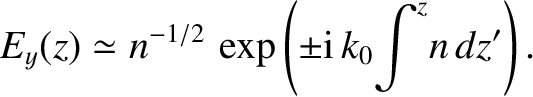
![$\lambda(z)= 2\pi/ [k_0\,n(z)]$](img1944.png) . Equations (6.17) and (6.18) also imply that the amplitude
of the wave gradually changes as it propagates. In fact, the amplitude of the electric
field component is inversely proportional to
. Equations (6.17) and (6.18) also imply that the amplitude
of the wave gradually changes as it propagates. In fact, the amplitude of the electric
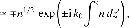
field component is inversely proportional to  , whereas the amplitude of the
magnetic field component is directly proportional to .
Note, however, that the energy
flux in the -direction, which is given by the the Poynting vector
, whereas the amplitude of the
magnetic field component is directly proportional to .
Note, however, that the energy
flux in the -direction, which is given by the the Poynting vector
 , remains constant (assuming that is predominately
real).
, remains constant (assuming that is predominately
real).
Of course, the WKB solutions (6.17) and (6.18) are only approximations. In reality,
a wave propagating through a medium in which the refractive index is a slowly
varying function of position is subject to a small amount of reflection.
However, it is easily demonstrated that the ratio of the reflected amplitude
to the incident amplitude is of order
 (Budden 1985). Thus, as long as
the refractive index varies on a much longer lengthscale than the wavelength
of the radiation, the reflected wave is negligibly small. This conclusion remains
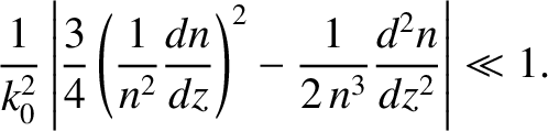
valid as long as the inequality (6.16) is satisfied.
This inequality obviously
breaks down in the vicinity of a point where
(Budden 1985). Thus, as long as
the refractive index varies on a much longer lengthscale than the wavelength
of the radiation, the reflected wave is negligibly small. This conclusion remains
valid as long as the inequality (6.16) is satisfied.
This inequality obviously
breaks down in the vicinity of a point where  . We would, therefore,
expect strong reflection of the incident wave from such a point.
Furthermore, the WKB solutions also break down at a
point where
. We would, therefore,
expect strong reflection of the incident wave from such a point.
Furthermore, the WKB solutions also break down at a
point where
 , because the amplitude of
  becomes
infinite.
becomes
infinite.