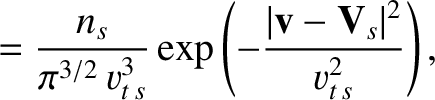
Suppose that the
species- and species-
 distribution functions are Maxwellian, but are characterized by different number densities, mean flow velocities, and kinetic
temperatures. Let us calculate the collision operator. Without loss of generality, we can choose to work in a frame of reference in which the species- mean flow velocity
is zero. It follows that
where
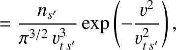
distribution functions are Maxwellian, but are characterized by different number densities, mean flow velocities, and kinetic
temperatures. Let us calculate the collision operator. Without loss of generality, we can choose to work in a frame of reference in which the species- mean flow velocity
is zero. It follows that
where
 and
and
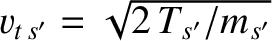 are the species- and species- thermal velocities, respectively. Moreover,
  ,
,  , and
, and  are the number density,
mean flow velocity, and temperature of species , whereas
are the number density,
mean flow velocity, and temperature of species , whereas  ,
,  , and
, and  are the corresponding quantities for
species
are the corresponding quantities for
species
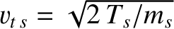
Given that
 is isotropic in velocity space, Equations (3.110) and (3.111) yield
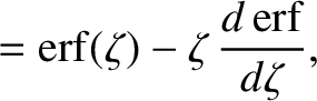
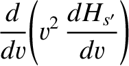
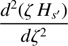
Making use of Equation (3.146), we obtain
where
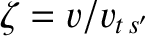 . Equation (3.149) can be integrated, subject to the boundary condition that
 remain finite at
 , to give
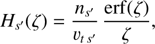 |
(3.151) |
where
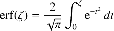 |
(3.152) |
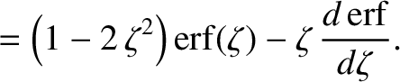
is an error function (Abramowitz and Stegun 1965). Hence, Equation (3.150) yields
 |
(3.153) |
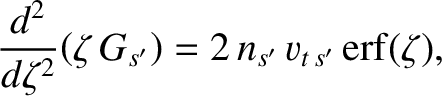
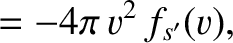
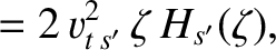
which can be integrated, subject to the constraint that  be finite at , to give
![$\displaystyle G_{s'}(\zeta) = \frac{n_{s'}\,v_{t\,{s'}}}{2\,\zeta}\left[\zeta\,\frac{d\,{\rm erf}}{d\zeta}+\left(1+2\,\zeta^{2}\right){\rm erf}(\zeta)\right].$](img909.png) |
(3.154) |
It follows that
where
Thus, Equation (3.112) yields
 |
![$\displaystyle = \frac{\gamma_{ss'}\,n_{s'}}{m_s\,m_{s'}}\,\frac{\partial}{\part...
...{v_\alpha\,v_\beta}{v^{2}}\right\}\frac{\partial f_s}{\partial v_\beta}\right].$](img918.png) |
(3.159) |
 |
(3.160) |
The previous two equations imply that
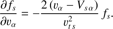
Suppose that the drift velocity, , is much smaller than the thermal velocity,  , of species- particles. In this case,
we can expand the distribution function (3.145) such that
, of species- particles. In this case,
we can expand the distribution function (3.145) such that
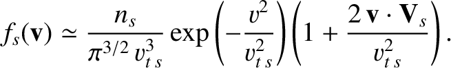 |
(3.161) |
Neglecting terms that are second order in
 , the previous two equations lead to the following final expression
for the collision operator for species with Maxwellian distribution functions:
where
, the previous two equations lead to the following final expression
for the collision operator for species with Maxwellian distribution functions:
where
 .
.


![$\displaystyle = \frac{n_{s'}\,v_{t\,{s'}}^{2}}{2\,v^{3}}\left\{-F_2(\zeta)\,\de...
...pha\beta}+ [F_2(\zeta)+2\,F_1(\zeta)]\,\frac{v_\alpha\,v_\beta}{v^{2}}\right\},$](img913.png)
![$\displaystyle = \frac{\gamma_{ss'}\,n_{s'}}{m_s\,m_{s'}}\,\frac{\partial}{\part...
...zeta)+2\,F_1(\zeta)]\,\frac{v_\alpha\,v_\beta}{v^{2}}\right\}\right]f_s\right).$](img920.png)

![$\displaystyle \left.\left.\phantom{===}-\frac{T_{s'}}{T_s}\,\frac{V_{s\,\beta}}...
...(\zeta)+2\,F_1(\zeta)]\,\frac{v_\alpha\,v_\beta}{v^{2}}\right\}\right]\right\},$](img925.png)