Next: Cold-Plasma Equations Up: Plasma Fluid Theory Previous: Magnetized Limit Contents
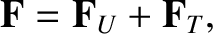
Let us consider a magnetized plasma. It is convenient to split the friction force
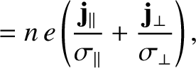
 into a component
  corresponding to resistivity, and a
component
corresponding to resistivity, and a
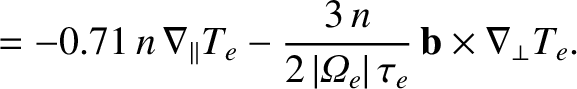
component  corresponding to the thermal force. Thus,
 |
(4.119) |
 |
 |
(4.120) |
 |
 |
(4.121) |
 is split
into a component
is split
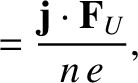
into a component  corresponding to the energy lost to the ions (in the
ion rest frame), a component
corresponding to the energy lost to the ions (in the
ion rest frame), a component  corresponding to work done by the friction
force , and a component
corresponding to work done by the friction
force , and a component  corresponding to work done by the
thermal force . Thus,
corresponding to work done by the
thermal force . Thus,
 |
(4.122) |
 |
 |
(4.123) |
 |
 |
(4.124) |
 into
a diffusive component
into
a diffusive component
 and a convective component
 .
Thus,
.
Thus,
 |
(4.125) |
 |
 |
(4.126) |
 |
 |
(4.127) |
Let us, first of all, consider the electron fluid equations, which can be written:
 |
 |
(4.128) |
   |
 |
(4.129) |
  |
 |
(4.130) |
 ,
,  ,
,  ,
,  ,
and
,
and
 , be typical values
of the particle density, the electron thermal velocity, the electron
mean-free-path, the magnetic field-strength, and the
electron gyroradius, respectively.
Suppose that the typical electron flow velocity is
, be typical values
of the particle density, the electron thermal velocity, the electron
mean-free-path, the magnetic field-strength, and the
electron gyroradius, respectively.
Suppose that the typical electron flow velocity is
 , and
the typical variation lengthscale is
, and
the typical variation lengthscale is  . Let
. Let
 |
 |
(4.131) |
 |
 |
(4.132) |
 |
 |
(4.133) |
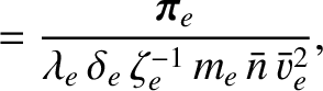
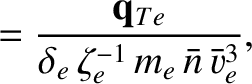
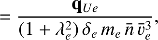
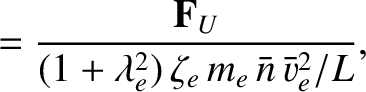
We define the following normalized quantities:
 |
 |
 |
 |
 |
 |
|
 |
 |
 |
 |
 |
 |
|
 |
 |
 |
 |
 |
 |
|
 |
 |
 |
 |
 |
 |
|
 |
 |
 |
 |
 |
 |
|
 |
 |
 |
 |
 |
 |
The normalization procedure is designed to make all hatted quantities
 .
The normalization of the electric field is chosen
such that the
.
The normalization of the electric field is chosen
such that the
 velocity is of similar magnitude to the electron fluid velocity. Note that the parallel viscosity
makes an
contribution to
velocity is of similar magnitude to the electron fluid velocity. Note that the parallel viscosity
makes an
contribution to
 , whereas the gyroviscosity
makes an
, whereas the gyroviscosity
makes an
 contribution, and the perpendicular viscosity only
makes an
contribution, and the perpendicular viscosity only
makes an
 contribution. Likewise, the parallel thermal
conductivity
makes an
contribution to
contribution. Likewise, the parallel thermal
conductivity
makes an
contribution to
 , whereas the cross
conductivity
makes an
contribution, and the perpendicular conductivity only
makes an
contribution. Similarly, the parallel components
of and
are
, whereas the perpendicular
components are
.
, whereas the cross
conductivity
makes an
contribution, and the perpendicular conductivity only
makes an
contribution. Similarly, the parallel components
of and
are
, whereas the perpendicular
components are
.
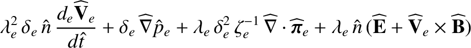
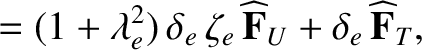
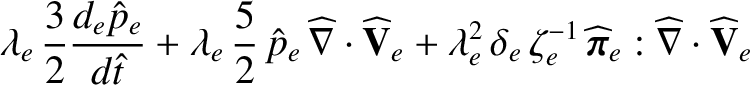
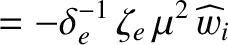
The normalized electron fluid equations take the form:
The only large or small (compared to unity) quantities in these equations are the parameters ,
,  ,
,  , and
, and  .
Here,
.
Here,
 . It is assumed that
 .
.
Let us now consider the ion fluid equations, which can be written:
 |
|
(4.137) |
  |
 |
(4.138) |
  |
 |
(4.139) |
,  ,
,  , ,
and
, ,
and
 , be typical values
of the particle density, the ion thermal velocity, the ion
mean-free-path, the magnetic field-strength, and the
ion gyroradius, respectively.
Suppose that the typical ion flow velocity is
, be typical values
of the particle density, the ion thermal velocity, the ion
mean-free-path, the magnetic field-strength, and the
ion gyroradius, respectively.
Suppose that the typical ion flow velocity is
 , and
the typical variation lengthscale is . Let
, and
the typical variation lengthscale is . Let
 |
 |
(4.140) |
 |
 |
(4.141) |
|
|
(4.142) |
We define the following normalized quantities:
|
|
 |
 |
|
|
|
|
|
|
 |
 |
 |
|
|
|
|
 |
|
 |
|
 |
 |
 |
 |
 |
 |
|
|
 |
|
 |
|
 |
As before, the normalization procedure is designed to make all hatted quantities
.
The normalization of the electric field is chosen
such that the
velocity is of similar magnitude to the ion fluid velocity. Note that the parallel viscosity
makes an
contribution to
 , whereas the gyroviscosity
makes an
, whereas the gyroviscosity
makes an
 contribution, and the perpendicular viscosity only
makes an
contribution, and the perpendicular viscosity only
makes an
 contribution. Likewise, the parallel thermal
conductivity
makes an
contribution to
contribution. Likewise, the parallel thermal
conductivity
makes an
contribution to
 , whereas the cross
conductivity
makes an
contribution, and the perpendicular conductivity only
makes an
contribution. Similarly, the parallel component
of is
, whereas the perpendicular
component is
, whereas the cross
conductivity
makes an
contribution, and the perpendicular conductivity only
makes an
contribution. Similarly, the parallel component
of is
, whereas the perpendicular
component is
 .
.
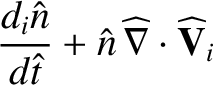
The normalized ion fluid equations take the form:
The only large or small (compared to unity) quantities in these equations are the parameters ,
,  ,
,  , and .
Here,
, and .
Here,
 .
.
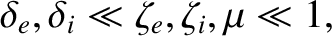
Let us adopt the ordering
 |
(4.146) |
and
as small parameters, and , , and as
.
In the second stage, we shall take note of the smallness of
, , and . Note that the parameters and
are “free ranging." In other words, they can be either large, small, or
.
In the initial stage of the
ordering procedure, the ion and electron
normalization schemes we have adopted become essentially
identical [because
 ], and
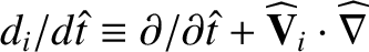
it is convenient to write
], and
it is convenient to write
 |
 |
(4.147) |
 |
 |
(4.148) |
 |
 |
(4.149) |
 |
 |
(4.150) |
 |
 |
(4.151) |
There are three fundamental orderings in plasma fluid theory.
The first fundamental ordering is
This corresponds to In other words, the fluid velocities are much greater than the respective thermal velocities. We also have Here, is conventionally termed the transit frequency, and is
the frequency with which fluid elements traverse the system. It is clear
that the transit frequencies are of approximately the same magnitudes as the gyrofrequencies
in this ordering. Keeping only the largest terms in Equations (4.134)–(4.136) and
(4.143)–(4.145), the Braginskii equations reduce to (in unnormalized form):
and
The factors in square brackets are just to remind us that the terms they precede
are smaller than the other terms in the equations (by the
corresponding factors inside
the
brackets).
is conventionally termed the transit frequency, and is
the frequency with which fluid elements traverse the system. It is clear
that the transit frequencies are of approximately the same magnitudes as the gyrofrequencies
in this ordering. Keeping only the largest terms in Equations (4.134)–(4.136) and
(4.143)–(4.145), the Braginskii equations reduce to (in unnormalized form):
and
The factors in square brackets are just to remind us that the terms they precede
are smaller than the other terms in the equations (by the
corresponding factors inside
the
brackets).
Equations (4.155)–(4.156) and (4.157)–(4.158) are called the cold-plasma equations, because
they can be obtained from the Braginskii equations by formally taking the
limit
 . Likewise, the ordering (4.152) is called
the cold-plasma approximation. The cold-plasma approximation
applies not only to cold plasmas, but also to very fast disturbances that
propagate through conventional plasmas. In particular,
the cold-plasma equations provide a good description of the propagation
of electromagnetic waves through plasmas. After all, electromagnetic
waves generally have very high velocities (i.e.,
. Likewise, the ordering (4.152) is called
the cold-plasma approximation. The cold-plasma approximation
applies not only to cold plasmas, but also to very fast disturbances that
propagate through conventional plasmas. In particular,
the cold-plasma equations provide a good description of the propagation
of electromagnetic waves through plasmas. After all, electromagnetic
waves generally have very high velocities (i.e.,  ),
which they impart to
plasma fluid elements, so there is usually
no difficulty satisfying the inequality (4.153).
),
which they impart to
plasma fluid elements, so there is usually
no difficulty satisfying the inequality (4.153).
The electron and ion pressures can be neglected in the cold-plasma limit, because the thermal velocities are much smaller than the fluid velocities. It follows that there is no need for an electron or ion energy evolution equation. Furthermore, the motion of the plasma is so fast, in this limit, that relatively slow “transport” effects, such as viscosity and thermal conductivity, play no role in the cold-plasma fluid equations. In fact, the only collisional effect that appears in these equations is resistivity.
The second fundamental ordering is
which corresponds to |
(4.160) |
Equations (4.161)–(4.163) and (4.164)–(4.165) are called the magnetohydrodynamical equations, or MHD equations, for short. Likewise, the ordering (4.159) is called the MHD approximation. The MHD equations are conventionally used to study macroscopic plasma instabilities possessing relatively fast growth-rates: for example, “sausage” modes and “kink” modes (Bateman 1978).
The electron and ion pressures cannot be neglected in the MHD limit, because the fluid velocities are similar in magnitude to the respective thermal velocities. Thus, electron and ion energy evolution equations are needed in this limit. However, MHD motion is sufficiently fast that “transport” effects, such as viscosity and thermal conductivity, are too slow to play a role in the MHD equations. In fact, the only collisional effects that appear in these equations are resistivity, the thermal force, and electron-ion collisional energy exchange.
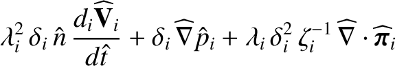
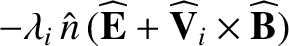
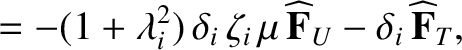
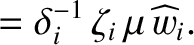
The third fundamental ordering is
which corresponds to |
(4.168) |
 is a typical drift (e.g., a curvature or grad-B
drift—see Chapter 2) velocity. In other words, the fluid velocities
are of similar magnitude to the respective drift velocities. Keeping only the
largest terms in Equations (3.113) and (3.116), the Braginskii equations reduce to
(in unnormalized form):
and
As before, the factors in square brackets remind us that the terms they
precede are larger, or smaller, than the other terms in the equations.
is a typical drift (e.g., a curvature or grad-B
drift—see Chapter 2) velocity. In other words, the fluid velocities
are of similar magnitude to the respective drift velocities. Keeping only the
largest terms in Equations (3.113) and (3.116), the Braginskii equations reduce to
(in unnormalized form):
and
As before, the factors in square brackets remind us that the terms they
precede are larger, or smaller, than the other terms in the equations.
Equations (4.169)–(4.171) and (4.172)–(4.174) are called the drift equations. Likewise, the ordering (4.167) is called the drift approximation. The drift equations are conventionally used to study equilibrium evolution, and the slow growing “micro-instabilities” that are responsible for turbulent transport in tokamaks. It is clear that virtually all of the original terms in the Braginskii equations must be retained in this limit.
In the following sections, we investigate the cold-plasma equations, the MHD equations, and the drift equations, in more detail.


![$\displaystyle = [\zeta]\,{\bf F}_U,$](img1438.png)
![$\displaystyle =- [\zeta]\,{\bf F}_U.$](img1440.png)

![$\displaystyle m_e \,n\,\frac{d_e {\bf V}_e}{dt} + \nabla p_e+ [\delta^{-1}]\,e\, n\,
({\bf E} + {\bf V}_e\times {\bf B})$](img1445.png)
![$\displaystyle = [\zeta]\,{\bf F}_U + {\bf F}_T,$](img1446.png)
![$\displaystyle = -[\delta^{-1}\,\zeta\,\mu^2]\,w_i,$](img1448.png)
![$\displaystyle m_i \,n\,\frac{d_i {\bf V}_i}{dt} + \nabla p_i - [\delta^{-1}]\, e \,n\,
({\bf E} + {\bf V}_i\times {\bf B})$](img1449.png)
![$\displaystyle =- [\zeta]\,{\bf F}_U
-{\bf F}_T,$](img1450.png)
![$\displaystyle =[\delta^{-1}\,\zeta\,\mu^2]\, w_i.$](img1452.png)

![$\displaystyle m_e \,n\,\frac{d_e {\bf V}_e}{dt} + [\delta^{-2}]\,\nabla p_e+
[\zeta^{-1}]\, \nabla\cdot$](img1456.png)

![$\displaystyle + [\delta^{-2}]\,e \,n\,
({\bf E} + {\bf V}_e\times {\bf B})$](img1458.png)
![$\displaystyle =[\delta^{-2}\,\zeta]\, {\bf F}_U + [\delta^{-2}]\,
{\bf F}_T,$](img1459.png)
![$\displaystyle \frac{3}{2}\frac{d_e p_e}{dt} + \frac{5}{2}\,p_e\,\nabla\cdot{\bf V}_e
+ [\zeta^{-1}]\,\nabla\cdot{\bf q}_{Te}
+ \nabla\cdot{\bf q}_{Ue}$](img1460.png)
![$\displaystyle =-[\delta^{-2}\,\zeta\,\mu^2]\, w_i
+[\zeta]\,w_U + w_T,$](img1461.png)
![$\displaystyle m_i \,n\,\frac{d_i {\bf V}_i}{dt} + [\delta^{-2}]\,\nabla p_i +
[\zeta^{-1}]\,\nabla\cdot$](img1462.png)

![$\displaystyle - [\delta^{-2}]\,e\, n\,
({\bf E} + {\bf V}_i\times {\bf B})$](img1464.png)
![$\displaystyle = -[\delta^{-2}\,\zeta]\, {\bf F}_U - [\delta^{-2}]\,{\bf F}_T,$](img1465.png)
![$\displaystyle \frac{3}{2}\frac{d_i p_i}{dt} + \frac{5}{2}\,p_i\,\nabla\cdot{\bf V}_i
+ [\zeta^{-1}]\,\nabla\cdot{\bf q}_i$](img1466.png)
![$\displaystyle = [\delta^{-2}\,\zeta\,\mu^2]\,W_i.$](img1467.png)