Next: Second Adiabatic Invariant Up: Charged Particle Motion Previous: Van Allen Radiation Belts Contents
 drift,
grad-
drift,
grad- drift, and curvature drift:
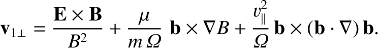 |
(2.108) |
drift, because this motion merely gives
rise to the convection of plasma within the magnetosphere, without generating a
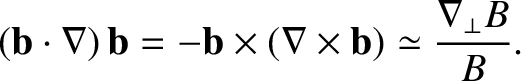
current. By contrast, there is a net current associated with grad- drift
and curvature drift. In the limit in which this current does not strongly
modify the ambient magnetic field (that is,
 ),
which is certainly the situation in the Earth's inner magnetosphere, we can write
),
which is certainly the situation in the Earth's inner magnetosphere, we can write
 |
(2.109) |
 |
(2.110) |
Although the perturbations to the Earth's magnetic field induced by the ring current are small, they are still detectable. In fact, the ring current causes a slight reduction in the Earth's magnetic field in equatorial regions. The size of this reduction is a good measure of the number of charged particles contained in the Van Allen belts. During the development of so-called geomagnetic storms, charged particles are injected into the Van Allen belts from the outer magnetosphere, giving rise to a sharp increase in the ring current, and a corresponding decrease in the Earth's equatorial magnetic field. These particles eventually precipitate out of the magnetosphere into the upper atmosphere at high terrestrial latitudes, giving rise to intense auroral activity, serious interference in electromagnetic communications, and, in extreme cases, disruption of electric power grids. The reduction in the Earth's magnetic field induced by the ring current is measured by the so-called Dst index, which is determined from hourly averages of the northward horizontal component of the terrestrial magnetic field recorded at four low-latitude observatories: Honolulu (Hawaii), San Juan (Puerto Rico), Hermanus (South Africa), and Kakioka (Japan). Figure 2.3 shows the Dst index for the month of March 1989. The very marked reduction in the index, centered on March 13, corresponds to one of the most severe geomagnetic storms experienced in recent decades. In fact, this particular storm was so severe that it tripped out the whole Hydro Québec electric distribution system, plunging more than 6 million customers into darkness. Most of Hydro Québec's neighboring systems in the United States came uncomfortably close to experiencing the same cascading power outage scenario. Incidentally, a reduction in the Dst index by 600 nT corresponds to a 2 percent reduction in the terrestrial magnetic field at the equator.
![\includegraphics[height=3.2in]{Chapter02/fig2_3.eps}](img482.png) |
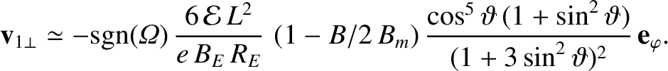
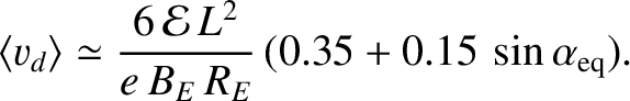
According to Equation (2.111), the precessional drift velocity of charged particles in the magnetosphere is a rapidly decreasing function of increasing latitude (in other words, the ring current is concentrated in the equatorial plane). Because charged particles typically complete many bounce orbits during a full circuit around the Earth, it is convenient to average Equation (2.111) over a bounce period to obtain the average drift velocity. This averaging can only be performed numerically. The final answer is well approximated by (Baumjohan and Treumann 1996)
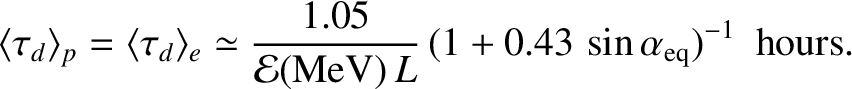
The average drift period (that is, the time required to perform a complete circuit around the Earth) is simply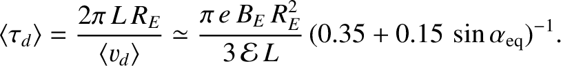 |
(2.113) |
 |
(2.114) |
 -shells.
Of course, charged particles only get a chance to complete a
full circuit around the Earth if the inner magnetosphere remains quiescent
on timescales of order an hour. This is, by no means, always the case.
-shells.
Of course, charged particles only get a chance to complete a
full circuit around the Earth if the inner magnetosphere remains quiescent
on timescales of order an hour. This is, by no means, always the case.
Finally, because the rest mass of an electron is  MeV, many
of the previous formulae require relativistic correction when applied to
MeV energy electrons.
Fortunately, however, there is no such problem for protons, whose rest mass
energy is
MeV, many
of the previous formulae require relativistic correction when applied to
MeV energy electrons.
Fortunately, however, there is no such problem for protons, whose rest mass
energy is  GeV.
GeV.