Next: Resonant Layers Up: Waves in Inhomogeneous Plasmas Previous: Cutoffs Contents
 , so that
in the immediate vicinity of this point, where
, so that
in the immediate vicinity of this point, where  . Here,
  is a small real constant. We introduce in our analysis principally
as a mathematical artifice to ensure that
is a small real constant. We introduce in our analysis principally
as a mathematical artifice to ensure that  remains single-valued and
finite. However, as will become clear later on, has a physical significance
in terms of the damping or the spontaneous excitation of waves.
remains single-valued and
finite. However, as will become clear later on, has a physical significance
in terms of the damping or the spontaneous excitation of waves.
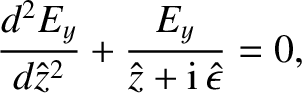
In the immediate vicinity of the resonance point, , Equations (6.3) and (6.29)
yield
 |
(6.31) |
 . This equation is
singular at the point
. This equation is
singular at the point
 .
Thus, it is necessary to
introduce a branch-cut into the complex-
.
Thus, it is necessary to
introduce a branch-cut into the complex- plane, so as to
ensure that
plane, so as to
ensure that
 is single-valued. If
 then the
branch-cut lies in the lower half-plane, whereas if
then the
branch-cut lies in the lower half-plane, whereas if
 then
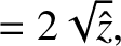
the branch-cut lies in the upper half-plane. (See Figure 6.1.) Suppose that the
argument of is 0 on the positive real -axis.
It follows that the argument of on the negative real -axis
is
then
the branch-cut lies in the upper half-plane. (See Figure 6.1.) Suppose that the
argument of is 0 on the positive real -axis.
It follows that the argument of on the negative real -axis
is  when
, and
when
, and  when
.
when
.
Let
 |
 |
(6.32) |
 |
 |
(6.33) |
 , Equation (6.30) transforms into
 |
(6.34) |
 and
and  ,
respectively. Thus, on the positive real -axis, we can write
the most general solution to Equation (6.30) in the form
where
,
respectively. Thus, on the positive real -axis, we can write
the most general solution to Equation (6.30) in the form
where  and
and  are two arbitrary constants.
Let
|
 |
(6.36) |
|
 |
(6.37) |
![$\displaystyle a = \exp\left[-{\rm i}\,\pi\,{\rm sgn}(\epsilon)\right].$](img1992.png) |
(6.38) |
 is zero on the negative real
-axis.
In the limit
, Equation (6.30) transforms into
is zero on the negative real
-axis.
In the limit
, Equation (6.30) transforms into
 |
(6.39) |
 and
and  ,
respectively. Thus, on the negative real -axis, we can write
the most general solution to Equation (6.30) in the form
where
,
respectively. Thus, on the negative real -axis, we can write
the most general solution to Equation (6.30) in the form
where  and
and  are two arbitrary constants.
The Bessel functions  ,
,  ,
,  , and
, and  are all perfectly
well-defined (i.e., analytic) for
complex arguments, so the two expressions (6.35) and (6.40) must, in fact, be
identical.
In particular, the constants and must somehow be related to the
constants and . In order to establish this relationship, it
is convenient to investigate the behavior of the expressions
(6.35) and (6.40) in the limit of small : that is,
are all perfectly
well-defined (i.e., analytic) for
complex arguments, so the two expressions (6.35) and (6.40) must, in fact, be
identical.
In particular, the constants and must somehow be related to the
constants and . In order to establish this relationship, it
is convenient to investigate the behavior of the expressions
(6.35) and (6.40) in the limit of small : that is,
 .
In this limit,
.
In this limit,
 is Euler's constant (Abramowitz and Stegun 1965), and is assumed to lie on the positive
real -axis. It follows, by a comparison of Equations (6.35), (6.40),
and (6.41)–(6.44), that the choice
is Euler's constant (Abramowitz and Stegun 1965), and is assumed to lie on the positive
real -axis. It follows, by a comparison of Equations (6.35), (6.40),
and (6.41)–(6.44), that the choice
 |
 |
(6.45) |
 |
 |
(6.46) |
In the limit
 ,
,
 |
 |
(6.47) |
 |
 |
(6.48) |
is assumed to lie on the negative real -axis.
It is clear that the  solution is unphysical, because it blows up
in the evanescent region
solution is unphysical, because it blows up
in the evanescent region
 . Thus, the coefficient in expression
(6.40) must be set to zero in order to prevent
from
blowing up as
. Thus, the coefficient in expression
(6.40) must be set to zero in order to prevent
from
blowing up as
 . According to Equation (6.45),
this constraint implies that
. According to Equation (6.45),
this constraint implies that
In the limit
,
is assumed to lie on the positive real -axis.
It follows from Equations (6.35), (6.49), (6.50), and (6.51) that, in the
non-evanescent region (
 ), the most general
physical solution takes the form
where
), the most general
physical solution takes the form
where  is an arbitrary constant.
Suppose that a plane electromagnetic wave, polarized in the
 -direction, is launched
from an antenna, located at large positive
-direction, is launched
from an antenna, located at large positive  , toward the resonance
point at .
It is assumed that
, toward the resonance
point at .
It is assumed that  at the launch point.
In the non-evanescent region,
at the launch point.
In the non-evanescent region,  , the wave can be
represented as a linear combination
of propagating WKB solutions:
, the wave can be
represented as a linear combination
of propagating WKB solutions:
 |
(6.53) |
 is the amplitude of the incident wave, and
  is the amplitude of
the reflected wave.
In the vicinity of the resonance point (i.e., small and positive,
which corresponds to large and positive),
the previous expression reduces to
A comparison of Equations (6.52) and (6.54) shows that if
then
is the amplitude of
the reflected wave.
In the vicinity of the resonance point (i.e., small and positive,
which corresponds to large and positive),
the previous expression reduces to
A comparison of Equations (6.52) and (6.54) shows that if
then
 . In other words, there is a reflected wave, but no incident wave.
This corresponds to the spontaneous excitation of waves in the vicinity of the
resonance. On the other hand, if
then
. In other words, there is a reflected wave, but no incident wave.
This corresponds to the spontaneous excitation of waves in the vicinity of the
resonance. On the other hand, if
then  . In other words,
there is an incident wave, but no reflected wave. This corresponds to the
total absorption of incident waves in the vicinity of the resonance.
It is clear that if
then represents some sort of
spontaneous wave excitation mechanism, whereas if
then
represents a wave absorption, or damping, mechanism.
We would normally expect plasmas to absorb incident wave energy, rather
than spontaneously emit waves, so we conclude that, under most circumstances,
, and resonances absorb incident waves without reflection.
. In other words,
there is an incident wave, but no reflected wave. This corresponds to the
total absorption of incident waves in the vicinity of the resonance.
It is clear that if
then represents some sort of
spontaneous wave excitation mechanism, whereas if
then
represents a wave absorption, or damping, mechanism.
We would normally expect plasmas to absorb incident wave energy, rather
than spontaneously emit waves, so we conclude that, under most circumstances,
, and resonances absorb incident waves without reflection.
![\includegraphics[height=3.26in]{Chapter06/fig6_1.eps}](img1980.png)


![$\displaystyle = -\frac{1}{\pi}\left[
1 -\left(\ln\vert\hat{z}\vert + 2\,\gamma-1\right)\hat{z}\,\right]+ {\cal O}\left(\hat{z}^{2}\right),$](img2009.png)
![$\displaystyle = \frac{1}{2}\left[
1 -\left( \ln\vert\hat{z}\vert + 2\,\gamma-1\...
... - {\rm i}\,{\rm arg}(a)\,
\hat{z}\,\right]
+ {\cal O}\left(\hat{z}^{2}\right),$](img2011.png)

![$\displaystyle = A'\,\left[{\rm sgn}(\epsilon) + 1\right]\,\hat{z}^{1/4}\,
\exp\left[
+{\rm i}\left(2\sqrt{\hat{z}} - \frac{3}{4}\,\pi\right)\right]$](img2028.png)
![$\displaystyle \phantom{=}+A'\,
\left[{\rm sgn}(\epsilon) - 1\right]\,\hat{z}^{1/4}\,\exp\left[
-{\rm i}\left(2\sqrt{\hat{z}} + \frac{3}{4}\,\pi\right)\right],$](img2029.png)
![$\displaystyle E_y(\hat{z}) \simeq (k_0 \,b)^{-1/2}\left[
E\,\hat{z}^{1/4}\exp\l...
...z}}\right)
+ F\,\hat{z}^{1/4}\exp\left(+{\rm i}\,2\sqrt{\hat{z}}\right)\right].$](img2033.png)