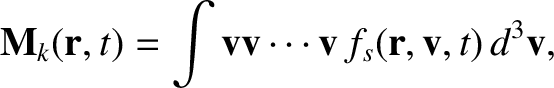
The  th velocity space moment of the (ensemble-averaged) distribution function
 is written
 |
(4.4) |
with factors of  . Clearly,
  is a tensor of rank (Riley 1974).
The set , for
 ,
can be viewed as an alternative description of the distribution function that uniquely specifies
,
can be viewed as an alternative description of the distribution function that uniquely specifies  when the latter is sufficiently smooth. For example,
a (displaced) Gaussian distribution function is uniquely specified by three
moments:
when the latter is sufficiently smooth. For example,
a (displaced) Gaussian distribution function is uniquely specified by three
moments:  , the vector
  , and the scalar formed by contracting
 .
.
The low-order moments all have simple physical interpretations.
First, we have the particle number density,
 |
(4.5) |
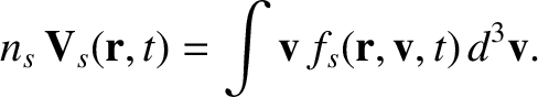
and the particle flux density,
 |
(4.6) |
The quantity  is, of course, the flow velocity. The constitutive relations, (3.1) and (3.2), are determined by these lowest
moments. In fact,
is, of course, the flow velocity. The constitutive relations, (3.1) and (3.2), are determined by these lowest
moments. In fact,
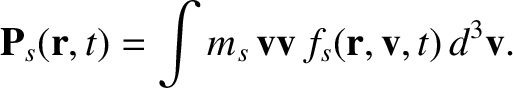
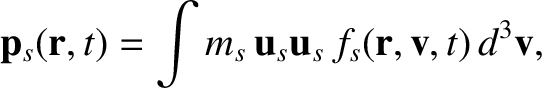
The second-order moment, describing the flow of momentum in the
laboratory frame, is called the stress tensor, and takes the form
 |
(4.9) |
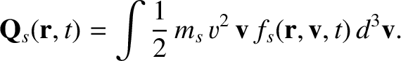
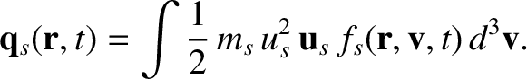
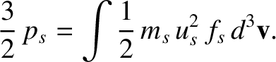
Finally, there is an important third-order moment
measuring the energy flux density,
 |
(4.10) |
It is often convenient to measure the second- and third-order moments in the rest-frame of the species under consideration. In this case, the
moments have different names. The stress tensor measured in the rest-frame
is called the pressure tensor,  , whereas the energy flux
density becomes the heat flux density,
, whereas the energy flux
density becomes the heat flux density,  . We introduce the
relative velocity,
. We introduce the
relative velocity,
 |
(4.11) |
in order to write
 |
(4.12) |
and
 |
(4.13) |
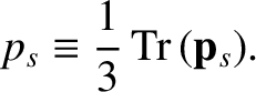
The trace of the pressure tensor measures the ordinary (or scalar) pressure,
 |
(4.14) |
In fact,
 is the kinetic energy density of species
  : that is,
 |
(4.15) |
In thermodynamic equilibrium, the distribution function becomes a Maxwellian
characterized by some temperature  , and Equation (4.15) yields
  . It
is, therefore, natural to define the (kinetic) temperature as
. It
is, therefore, natural to define the (kinetic) temperature as
 |
(4.16) |
Of course, the moments measured in the two different frames are related.
By direct substitution, it is easily verified that