Next: Constant- Magnetic Islands Up: Magnetic Reconnection Previous: Tearing Modes Contents
 limit,
  .
In order to determine how this solution is modified when the constant- approximation breaks down, we need to find a
solution that is valid as
.
In order to determine how this solution is modified when the constant- approximation breaks down, we need to find a
solution that is valid as
 .
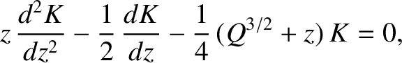
Now, when expanded to
.
Now, when expanded to
 , the most
general small-
, the most
general small- asymptotic solution of Equation (9.45) takes the form
As before,
asymptotic solution of Equation (9.45) takes the form
As before,  and
and  are independent of , and it is assumed that
  .
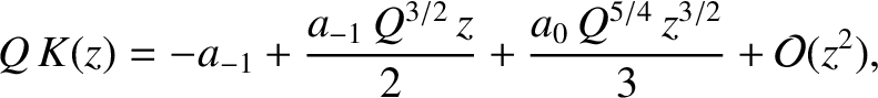
Let
Equation (9.45) transforms to give
As is clear from Equations (9.67) and (9.68), the most general small- asymptotic solution of the
previous equation is
.
Let
Equation (9.45) transforms to give
As is clear from Equations (9.67) and (9.68), the most general small- asymptotic solution of the
previous equation is
Let
 |
(9.71) |
![\includegraphics[height=3.in]{Chapter09/fig9_4.eps}](img3437.png) |
Let
 |
(9.74) |
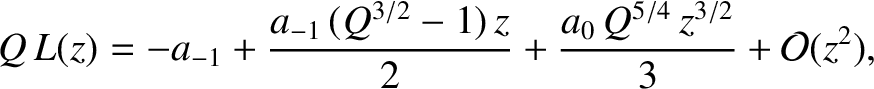
 is a confluent hypergeometric function of the second kind (Abramowitz and Stegun 1965),
![$\displaystyle L(z) =U\!\left[\frac{1}{4}\,(Q^{3/2}-1),-\frac{1}{2},z\right],$](img3441.png) |
(9.77) |
 asymptotic expansion (Abramowitz and Stegun 1965)
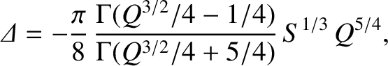
Comparing Equations (9.49), (9.76), and (9.78), we obtain (Coppi, et al., 1976; Pegoraro and Schep 1986)
where use has been made of some elementary properties of gamma functions (Abramowitz and Stegun 1965).
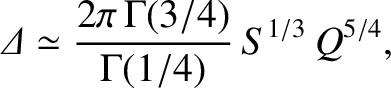
In the constant- limit, , the previous expression reduces to
which is consistent with Equation (9.58).
asymptotic expansion (Abramowitz and Stegun 1965)
Comparing Equations (9.49), (9.76), and (9.78), we obtain (Coppi, et al., 1976; Pegoraro and Schep 1986)
where use has been made of some elementary properties of gamma functions (Abramowitz and Stegun 1965).
In the constant- limit, , the previous expression reduces to
which is consistent with Equation (9.58).
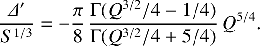
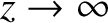
When combined with the matching condition (9.42), Equation (9.79) yields the dispersion relation
This dispersion relation is illustrated in Figure 9.4. It can be seen that in the constant- regime,
 , in accordance with standard tearing mode theory. (See Section 9.5.) On the other hand,
in the
non-constant- regime,
, in accordance with standard tearing mode theory. (See Section 9.5.) On the other hand,
in the
non-constant- regime,
 .
.
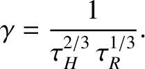
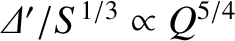
The general dispersion relation (9.81) implies that the growth-rate of a tearing mode does not continue
to increase indefinitely as the tearing stability index,
 , becomes larger and larger, which is the prediction of the constant-
dispersion relation (9.60). Instead, when
exceeds a critical value that is
of order
, becomes larger and larger, which is the prediction of the constant-
dispersion relation (9.60). Instead, when
exceeds a critical value that is
of order  (implying the breakdown of the constant- approximation), the growth-rate saturates at the
value
(implying the breakdown of the constant- approximation), the growth-rate saturates at the
value
 |
(9.82) |

![$\displaystyle L(z) = -\pi\left[\frac{1-(1/2)\,(Q^{3/2}-1)\,z}
{{\Gamma}[(5+Q^{3...
...-\frac{z^{3/2}}
{{\Gamma}[(Q^{3/2}-1)/4]\,{\Gamma}(5/2)} +{\cal O}(z^2)\right].$](img3442.png)