Next: Asymptotic Matching Up: Magnetic Reconnection Previous: Reduced-MHD Equations Contents
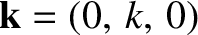
 is a unit vector parallel to the
  -axis. The equilibrium plasma flow is assumed to be zero.
The current sheet consists of filaments that run parallel to the
-axis. The equilibrium plasma flow is assumed to be zero.
The current sheet consists of filaments that run parallel to the  -axis. As illustrated in Figure 9.1, the
sheet is centered on the plane
-axis. As illustrated in Figure 9.1, the
sheet is centered on the plane  , and is of thickness
  in the
  -direction. The magnetic field
generated by the current sheet is parallel to the -axis, of magnitude
-direction. The magnetic field
generated by the current sheet is parallel to the -axis, of magnitude  , and switches direction
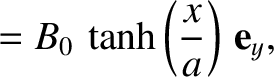
across the sheet. In other words,
, and switches direction
across the sheet. In other words,
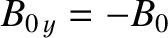 for
for 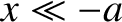 , and
, and
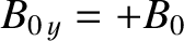 for
for 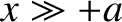 .
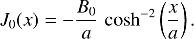
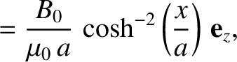
Note that
.
Note that
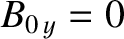 at the center of the sheet, .
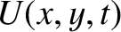
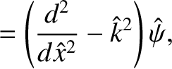
Consider a small perturbation to the aforementioned current sheet that varies periodically in the -direction with
wavelength  . The wavevector of the perturbation is therefore
 . It follows that the
perturbation satisfies the shear-Alfvén resonance condition,
. It follows that the
perturbation satisfies the shear-Alfvén resonance condition,
 , at .
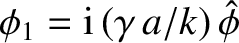
We can write
, at .
We can write
 is the growth-rate of the perturbation, and
  ,
,  ,
,  , and
, and  are all
considered to be small (compared to equilibrium quantities) quantities.
are all
considered to be small (compared to equilibrium quantities) quantities.
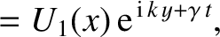
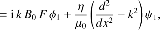
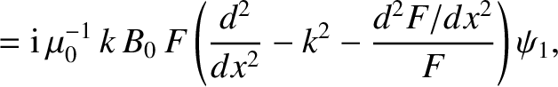
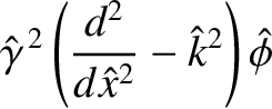
Substituting Equations (9.18)–(9.21) into the reduced-MHD equations, (9.11)–(9.14), making use of Equation (9.15), and only retaining terms that are first order in small quantities, we obtain the linearized reduced-MHD equations:
where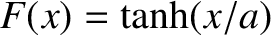 .
.
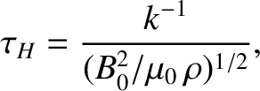
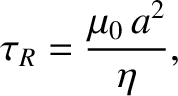
It is helpful to define the hydromagnetic timescale,
which is the typical time required for a shear-Alfvén wave to propagate a wavelength parallel to the-axis, as well as the resistive diffusion timescale,
which is the typical time required for magnetic flux to diffuse across the current sheet in the -direction. The effective
Lundquist number for the problem is
 |
(9.26) |
Let
 ,
,
 ,
,
 ,
,
 ,
and
,
and
 . The dimensionless, normalized
versions of the linearized reduced-MHD equations, (9.22) and (9.23), become
. The dimensionless, normalized
versions of the linearized reduced-MHD equations, (9.22) and (9.23), become
 and
and
 . Our normalization scheme is designed such that, throughout the
bulk of the plasma,
. Our normalization scheme is designed such that, throughout the
bulk of the plasma,
 , and the only other quantities in the previous two equations whose magnitudes differ substantially
from unity are
, and the only other quantities in the previous two equations whose magnitudes differ substantially
from unity are
 and
and
 .
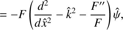
The term on the right-hand side of Equation (9.27) represents plasma resistivity, whereas the term on the left-hand side of Equation (9.28). represents plasma inertia.
The shear-Alfvén resonance condition,
.
The term on the right-hand side of Equation (9.27) represents plasma resistivity, whereas the term on the left-hand side of Equation (9.28). represents plasma inertia.
The shear-Alfvén resonance condition,
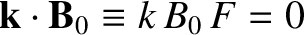 , reduces to
  .
.


![\includegraphics[height=2.9in]{Chapter09/fig9_1.eps}](img3285.png)
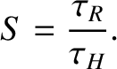
![$\displaystyle = -B_0\,a\,\ln\left[\cosh\left(\frac{x}{a}\right)\right] + \psi_1(x)\,{\rm e}^{\,{\rm i}\,k\,y+\gamma\,t},$](img3291.png)