Next: Exercises
Up: Collisions
Previous: Rosenbluth Potentials
Collision Times
Consider collisions between particles of type  (with number density
  and mass
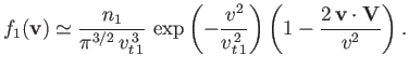
  ), possessing the Maxwellian distribution function
![$\displaystyle f_1({\bf v})=n_1\left(\frac{m_1}{2\pi\,T}\right)^{3/2}\exp\left[-\frac{m_1\,({\bf v}-{\bf V})^2}{2\,T}\right],$](img939.png) |
(3.167) |
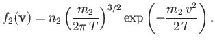
and particles of type  (with number density
  and mass
  ), possessing the Maxwellian distribution function
 |
(3.168) |
Here,  is the common temperature of the two species, and
  is the mean drift velocity of species
relative to species
.
As we saw in the previous section, collisions with particles of type
give rise to a velocity-dependent force acting on individual particles of
type
. This force takes the form [see Equation (3.165)]
is the mean drift velocity of species
relative to species
.
As we saw in the previous section, collisions with particles of type
give rise to a velocity-dependent force acting on individual particles of
type
. This force takes the form [see Equation (3.165)]
![$\displaystyle {\bf R}_{12} =- \frac{\gamma_{12}\,n_2}{m_2}\left[-\frac{F_2(\zet...
...3}\,{\bf V} + \frac{3\,F_3(\zeta)}{v^5}\,({\bf v}\cdot{\bf V})\,{\bf v}\right],$](img941.png) |
(3.169) |
where
 and
and
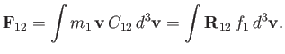
 . The net force per unit volume acting on type
particles due to
collisions with type
particles is thus
. The net force per unit volume acting on type
particles due to
collisions with type
particles is thus
 |
(3.170) |
Suppose that the drift velocity,
, is much smaller than the thermal velocity,
 , of type
particles.
In this case, we can write
, of type
particles.
In this case, we can write
 |
(3.171) |
Hence, Equations (3.169) and (3.170) yield
 |
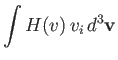
![$\displaystyle = -\frac{\gamma_{12}\,n_1\,n_2}{\pi^{3/2}\,m_2\,v_{t\,1}^{\,3}}\i...
...(\zeta)}{v^3}\,V_i + \frac{3\,F_3(\zeta)}{v^5}\,v_k\,V_k\,v_i\right]d^3{\bf v}.$](img947.png) |
|
| |
|
(3.172) |
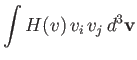
However, it follows from symmetry that
where  is a general function. Hence, Equation (3.172) reduces to
![$\displaystyle {\bf F}_{12} = -\frac{\gamma_{12}\,n_1\,n_2\,{\bf V}}{\pi^{3/2}\,...
...v_{t\,1}^{\,2}}\right)\left[\frac{F_3(\zeta)-F_2(\zeta)}{v^3}\right]d^3{\bf v}.$](img953.png) |
(3.176) |
It follows from Equations (3.151) and (3.152) that
 |
(3.177) |
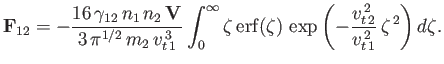
Integration by parts gives
![$\displaystyle {\bf F}_{12} = -\frac{16\,\gamma_{12}\,n_1\,n_2\,{\bf V}}{3\,\pi\...
...-\left(1+\frac{v_{t\,2}^{\,2}}{v_{t\,1}^{\,2}}\right) \zeta^{\,2}\right]d\zeta,$](img955.png) |
(3.178) |
which reduces to
![$\displaystyle {\bf F}_{12} = -\left[\frac{8\,\gamma_{12}\,n_1\,n_2}{3\,\pi^{1/2}\,m_2\,v_{t\,2}^{\,2}\,(v_{t\,1}^{\,2}+v_{t\,2}^{\,2})^{1/2}}\right]{\bf V}.$](img956.png) |
(3.179) |
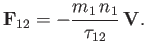
The collision time,  , associated with collisions of particles of type
with particles of type
, is conventionally
defined via the following equation,
, associated with collisions of particles of type
with particles of type
, is conventionally
defined via the following equation,
 |
(3.180) |
According to this definition, the collision time is the time required for collisions with particles of type
to decelerate particles of
type
to such an extent that the mean drift velocity of the latter particles with respect to the former is eliminated. At the individual
particle level, the collision time is the mean time required for the direction of motion of an individual type
particle to deviate through
approximately  as a consequence of collisions with particles of type
.
According to Equations (3.112) and (3.179),
we can write
as a consequence of collisions with particles of type
.
According to Equations (3.112) and (3.179),
we can write
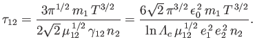 |
(3.181) |
Consider a quasi-neutral plasma consisting of electrons of mass  , charge
  , and number density
  , and ions
of mass
, and ions
of mass  , charge
  , and number density
  . Let the two species both have Maxwellian distributions characterized by a
common temperature
, and a small relative drift velocity. It follows, from the previous analysis, that we can
identify four different collision times. First, the electron-electron collision time,
. Let the two species both have Maxwellian distributions characterized by a
common temperature
, and a small relative drift velocity. It follows, from the previous analysis, that we can
identify four different collision times. First, the electron-electron collision time,
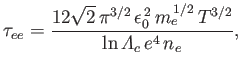 |
(3.182) |
which is the mean time required for the direction of motion of an individual electron to deviate through
approximately
as a consequence of collisions with other electrons.
Second, the electron-ion collision time,
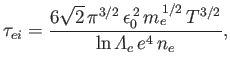 |
(3.183) |
which is the mean time required for the direction of motion of an individual electron to deviate through
approximately
as a consequence of collisions with ions.
Third, the ion-ion collision time,
 |
(3.184) |
which is the mean time required for the direction of motion of an individual ion to deviate through
approximately
as a consequence of collisions with other ions.
Finally, the ion-electron collision time,
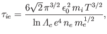 |
(3.185) |
which is the mean time required for the direction of motion of an individual ion to deviate through
approximately
as a consequence of collisions with electrons. Note that these collision times are not all
of the same magnitude, as a consequence of the large difference between the electron and ion masses.
In fact,
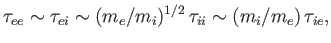 |
(3.186) |
which implies that electrons scatter electrons (through
) at about the same rate that ions scatter electrons, but that ions scatter ions
at a significantly lower rate than ions scatter electrons, and, finally, that electrons scatter ions at a significantly lower rate than ions scatter ions.
The collision frequency is simply the inverse of the collision time. Thus, the electron-electron collision frequency
is written
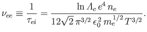 |
(3.187) |
Given that
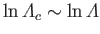 (see Section 3.10), where
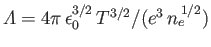 is the
plasma parameter (see Section 1.6),
we obtain the estimate (see Section 1.7)
is the
plasma parameter (see Section 1.6),
we obtain the estimate (see Section 1.7)
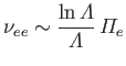 |
(3.188) |
where
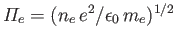 is the electron plasma frequency (see Section 1.4).
Likewise, the ion-ion collision frequency is such that
is the electron plasma frequency (see Section 1.4).
Likewise, the ion-ion collision frequency is such that
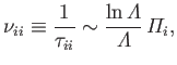 |
(3.189) |
where
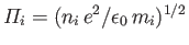 is the ion plasma frequency.
Next: Exercises
Up: Collisions
Previous: Rosenbluth Potentials
Richard Fitzpatrick
2016-01-23