Next: Energy Density Within Dielectric
Up: Electrostatics in Dielectric Media
Previous: Boundary Conditions for and
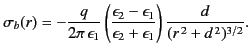
Consider a point charge  embedded in a semi-infinite dielectric medium of dielectric constant
 , and located a distance
  from a plane interface that
separates the first medium from another semi-infinite dielectric medium of
dielectric constant
from a plane interface that
separates the first medium from another semi-infinite dielectric medium of
dielectric constant
 . Suppose that the interface coincides with the plane
  .
We need to solve
.
We need to solve
 |
(512) |
in the region  ,
,
 |
(513) |
in the region  , and
, and
 |
(514) |
everywhere, subject to the following constraints at
:
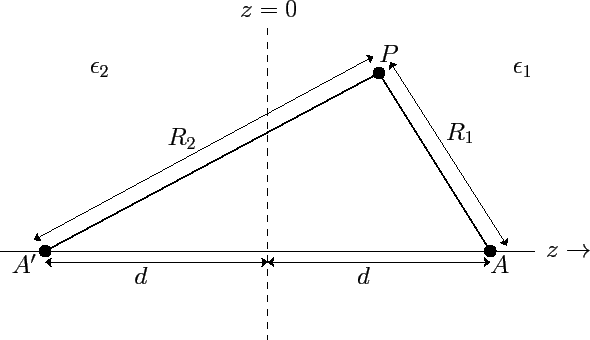
Figure 1:
The method of images for a plane interface between two dielectric media.
 |
In order to solve this problem, we shall employ a slightly modified form of
the well-known method of images. Because
 everywhere,
the electric field can be written in terms of a scalar potential: that is,
everywhere,
the electric field can be written in terms of a scalar potential: that is,
 . Consider the region
.
Let us assume that the scalar potential in this region is the same as
that obtained when the whole of space is filled with dielectric of dielectric constant
, and, in addition to the real charge
at position
. Consider the region
.
Let us assume that the scalar potential in this region is the same as
that obtained when the whole of space is filled with dielectric of dielectric constant
, and, in addition to the real charge
at position  ,
there is a second charge
,
there is a second charge  at the image position
  . (See Figure 1.)
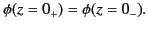
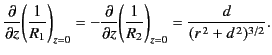
If this is the case then the potential at some point
. (See Figure 1.)
If this is the case then the potential at some point  in the region
is given by
in the region
is given by
 |
(518) |
where
 and
and
 . Here,
  ,
,  ,
,  are conventional cylindrical
coordinates.
Note that the potential (519) is clearly a solution of Equation (513) in
the region
: that is, it satisfies
are conventional cylindrical
coordinates.
Note that the potential (519) is clearly a solution of Equation (513) in
the region
: that is, it satisfies
 , with the
appropriate singularity at the position of the point charge
.
, with the
appropriate singularity at the position of the point charge
.
Consider the region
. Let us assume that the scalar potential in this
region is the same as that obtained when the whole of space is filled
with a dielectric medium of dielectric constant
, and a charge  is located at the point
. If this is the case then the potential in this region is
given by
is located at the point
. If this is the case then the potential in this region is
given by
 |
(519) |
The above potential is clearly a solution of Equation (514) in the region
: that is, it satisfies
, with
no singularities.
It now remains to choose
and
in such a manner that the constraints (516)-(518) are satisfied. The constraints (517) and
(518) are obviously satisfied if the scalar potential is continuous
across the interface between the two media: that is,
 |
(520) |
The constraint (516) implies a jump in the normal derivative
of the scalar potential across the interface. In fact,
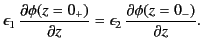 |
(521) |
The first matching condition yields
 |
(522) |
whereas the second gives
 |
(523) |
Here, use has been made of
 |
(524) |
Equations (523) and (524) imply that
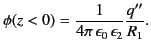
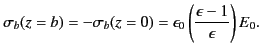
The polarization charge density is given by
 , However,
 inside either dielectric, which implies that
 |
(527) |
except at the point charge
.
Thus, there is zero bound charge density in either dielectric
medium. At the interface,  jumps discontinuously,
 |
(528) |
This implies that there is a bound charge sheet on the interface
between the two dielectric media. In fact, it follows from Equation (498) that
 |
(529) |
where
 is a unit normal to the interface pointing from
medium 1 to medium 2 (i.e., along the positive
-axis).
Because
is a unit normal to the interface pointing from
medium 1 to medium 2 (i.e., along the positive
-axis).
Because
 |
(530) |
in either medium, it is easily demonstrated that
 |
(531) |
In the limit
 , the dielectric
behaves like a conducting medium (i.e.,
, the dielectric
behaves like a conducting medium (i.e.,
 in the region
), and the bound surface charge density
on the interface approaches that obtained in the case when the plane
coincides with a conducting surface.
in the region
), and the bound surface charge density
on the interface approaches that obtained in the case when the plane
coincides with a conducting surface.
The above argument can easily be generalized to deal with problems
involving multiple point
charges in the presence of multiple dielectric media whose
interfaces form parallel planes.
Consider a second boundary value problem in which a slab of dielectric, of dielectric constant  , lies between the planes
and
, lies between the planes
and  . Suppose that this slab is placed in a uniform
-directed
electric field of strength
. Suppose that this slab is placed in a uniform
-directed
electric field of strength  . Let us calculate the field-strength
  inside
the slab.
inside
the slab.
Because there are no free charges, and this is essentially a one-dimensional problem, it
is clear from Equation (501) that the electric displacement  is the
same in both the dielectric slab and the surrounding vacuum.
In the vacuum region,
is the
same in both the dielectric slab and the surrounding vacuum.
In the vacuum region,
 , whereas
 in the dielectric. It follows that
 |
(532) |
In other words, the electric field inside the slab is reduced by
polarization charges.
As before, there is zero polarization charge density inside the dielectric.
However, there is a uniform bound charge sheet on both surfaces of
the slab. It is easily demonstrated that
 |
(533) |
In the limit
 , the slab acts like a conductor, and
 .
.
Let us now generalize this result. Consider a dielectric medium whose
dielectric constant
varies with
. The medium is assumed to
be of finite extent, and to be surrounded by a vacuum. It follows
that
 as
as
 . Suppose that this dielectric is
placed in a uniform
-directed electric field of strength
. What is the
field
. Suppose that this dielectric is
placed in a uniform
-directed electric field of strength
. What is the
field  inside the dielectric?
We know that the electric displacement inside the dielectric is
given by
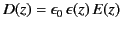 . We also know from
Equation (501) that, because there are no free charges, and this is
essentially a one-dimensional problem,
. We also know from
Equation (501) that, because there are no free charges, and this is
essentially a one-dimensional problem,
![$\displaystyle \frac{d D(z)}{dz} = \epsilon_0\, \frac{d [\epsilon(z)\, E(z)]}{d z} = 0.$](img1143.png) |
(534) |
Furthermore,
 as
.
It follows that
as
.
It follows that
 |
(535) |
Thus, the electric field is inversely proportional to the
dielectric constant of the medium. The bound
charge density within the medium is given by
![$\displaystyle \rho_b = \epsilon_0 \,\frac{d E(z)}{d z} = \epsilon_0\, E_0\frac{d}{dz} \!\left[\frac{1}{\epsilon(z)}\right].$](img1146.png) |
(536) |
Consider a third, and final, boundary value problem in which a dielectric sphere of radius  , and dielectric constant
, is placed in a
-directed electric field of strength
(in the absence of the sphere). Let us calculate the electric field inside
and around the sphere.
, and dielectric constant
, is placed in a
-directed electric field of strength
(in the absence of the sphere). Let us calculate the electric field inside
and around the sphere.
Because this is a static problem, we can write
.
There are no free charges, so Equations (501) and (505) imply that
 |
(537) |
everywhere. The matching conditions (510) and (512) reduce to
Furthermore,
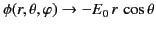 |
(540) |
as
 : that is, the electric field asymptotes to uniform
-directed field of strength
far from the
sphere. Here,
,
,
: that is, the electric field asymptotes to uniform
-directed field of strength
far from the
sphere. Here,
,
,  are spherical
coordinates centered on the sphere.
are spherical
coordinates centered on the sphere.
Let us search for an axisymmetric solution,
 . Because the
solutions to Poisson's equation are unique, we know
that if we can find such a solution that satisfies all of
the boundary conditions then we can be sure that this is the
correct solution. Equation (538) reduces to
. Because the
solutions to Poisson's equation are unique, we know
that if we can find such a solution that satisfies all of
the boundary conditions then we can be sure that this is the
correct solution. Equation (538) reduces to
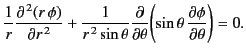 |
(541) |
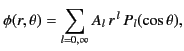
Straightforward separation of the variables yields (see Section 3.7)
![$\displaystyle \phi(r,\theta) = \sum_{l=0,\infty}\left[A_l \,r^{\,l} + B_l \,r^{\,-(l+1)}\right] P_l(\cos\theta),$](img1157.png) |
(542) |
where  is a non-negative
integer, the
is a non-negative
integer, the  and
and  are arbitrary constants, and the
  are Legendre polynomials. (See Section 3.2.)
The Legendre polynomials form a complete set of angular functions, and
it is easily demonstrated
that the  and the
 form a complete set of
radial functions. It follows that Equation (543), with the
and
unspecified, represents a completely general (single-valued) axisymmetric solution
to Equation (538). It remains to determine the values of the
and
that
are consistent with the boundary conditions.
form a complete set of
radial functions. It follows that Equation (543), with the
and
unspecified, represents a completely general (single-valued) axisymmetric solution
to Equation (538). It remains to determine the values of the
and
that
are consistent with the boundary conditions.
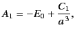
Let us divide space into the regions  and
and  . In the former
region
. In the former
region
 |
(543) |
where we have rejected the
radial solutions because they diverge
unphysically as
.
In the latter
region
![$\displaystyle \phi(r,\theta) = \sum_{l=0,\infty}\left[B_l\,r^{\,l} + C_l \,r^{\,-(l+1)}\right]P_l(\cos \theta).$](img1164.png) |
(544) |
However, it is clear from the boundary condition (541)
that the only non-vanishing
is  . This follows because
 . The boundary condition
(540) [which can be integrated to give
. The boundary condition
(540) [which can be integrated to give
 for a potential that is single-valued in
] gives
for a potential that is single-valued in
] gives
 |
(545) |
and
 |
(546) |
for  . Note that it is appropriate to match the coefficients of
the
. Note that it is appropriate to match the coefficients of
the
 because these functions are mutually orthogonal. (See Section 3.2.)
The boundary condition (539) yields
because these functions are mutually orthogonal. (See Section 3.2.)
The boundary condition (539) yields
 |
(547) |
and
 |
(548) |
for
. Equations (547) and (549) give
 for
. Equations (546) and (548) reduce to
for
. Equations (546) and (548) reduce to
The solution to the problem is therefore
 |
(551) |
for
, and
 |
(552) |
for
.
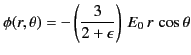
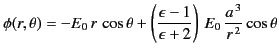
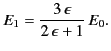
Equation (552) is the potential of a uniform
-directed electric
field of strength
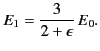 |
(553) |
Note that  , provided that
 . Thus, the electric
field-strength is reduced inside the dielectric sphere due to
partial shielding
by polarization charges. Outside the sphere, the potential is
equivalent to that of the applied field
, plus the field of
an electric dipole (see Section 2.7), located at the origin, and directed along the
-axis, whose dipole moment is
. Thus, the electric
field-strength is reduced inside the dielectric sphere due to
partial shielding
by polarization charges. Outside the sphere, the potential is
equivalent to that of the applied field
, plus the field of
an electric dipole (see Section 2.7), located at the origin, and directed along the
-axis, whose dipole moment is
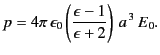 |
(554) |
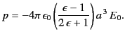
This dipole moment can be interpreted as the volume integral of the
polarization  over the sphere. The polarization is
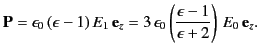 |
(555) |
Because the polarization is uniform there is
zero bound charge density inside the sphere.
However, there is a bound charge sheet on the surface of the
sphere, whose density
is given by
 [see Equation (530)]. It follows that
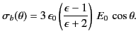 |
(556) |
The problem of a dielectric cavity of radius
inside a dielectric medium
of dielectric constant
, and in the presence of an applied electric field
, parallel to the
-axis, can be treated in much the same manner as
that of a dielectric sphere. In fact, it is easily demonstrated
that the results for the cavity can be obtained from those for the sphere by making the
transformation
 . Thus, the field
inside the cavity is uniform, parallel to the
-axis, and of magnitude
. Thus, the field
inside the cavity is uniform, parallel to the
-axis, and of magnitude
 |
(557) |
Note that  , provided that
. The field outside the
cavity is the original field, plus that of a
-directed dipole, located
at the
origin, whose dipole moment is
, provided that
. The field outside the
cavity is the original field, plus that of a
-directed dipole, located
at the
origin, whose dipole moment is
 |
(558) |
Here, the negative sign implies that the dipole points in the opposite
direction to
the external field.
Next: Energy Density Within Dielectric
Up: Electrostatics in Dielectric Media
Previous: Boundary Conditions for and
Richard Fitzpatrick
2014-06-27