Next: Axisymmetric Charge Distributions
Up: Potential Theory
Previous: Poisson's Equation in Spherical
Multipole Expansion
Consider a bounded charge distribution that lies inside the sphere  . It follows that
  in the region
  . According to the previous three equations, the electrostatic potential in the region
takes the form
. According to the previous three equations, the electrostatic potential in the region
takes the form
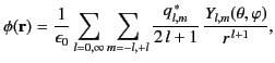 |
(339) |
where the
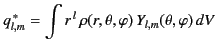 |
(340) |
are known as the multipole moments of the charge distribution
 . Here, the integral is over all space.
Incidentally, the type of expansion specified in Equation (340) is called a multipole expansion.
. Here, the integral is over all space.
Incidentally, the type of expansion specified in Equation (340) is called a multipole expansion.
The most important
 are those corresponding to
  ,
,  , and
, and  , which are known as monopole, dipole,
and quadrupole moments, respectively. For each
, which are known as monopole, dipole,
and quadrupole moments, respectively. For each  , the multipole moments
, for
, the multipole moments
, for
 to
to  , form an
th-rank tensor with
, form an
th-rank tensor with  components.
However, Equation (310) implies that
components.
However, Equation (310) implies that
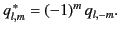 |
(341) |
Hence, only  of these components are independent.
For
, there is only one monopole moment. Namely,
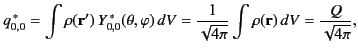 |
(342) |
where  is the net charge contained in the distribution, and use has been made of Equation (312). It follows from Equation (340) that, at sufficiently large
  , the charge
distribution acts like a point charge
situated at the origin. That is,
, the charge
distribution acts like a point charge
situated at the origin. That is,
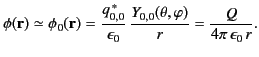 |
(343) |
By analogy with Equation (195), the dipole moment of the charge distribution is written
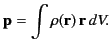 |
(344) |
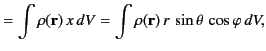
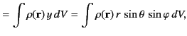
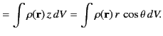
The three Cartesian components of this vector are
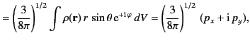
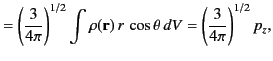
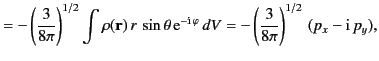
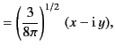
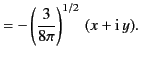
On the other hand, the spherical components of the dipole moment take the form
where use has been made of Equations (313)-(315).
It can be seen that the three spherical dipole moments are independent linear combinations of the three Cartesian moments. The potential
associated with the dipole moment is
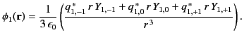 |
(351) |
However, from Equations (313)-(315),
Hence,
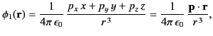 |
(355) |
in accordance with Equation (200). Note, finally, that if the net charge,
, contained in the distributions is non-zero then it is always possible to
choose the origin of the coordinate system in such a manner that
 .
.
The Cartesian components of the quadrupole tensor are defined
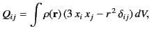 |
(356) |
for  ,
,  ,
,  ,
,  . Here,
  ,
,  , and
, and  . Incidentally, because the quadrupole tensor is symmetric (i.e.,
 )
and traceless (i.e.,
)
and traceless (i.e.,
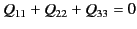 ), it only possesses five independent Cartesian components.
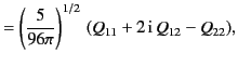
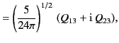
The five spherical components of the quadrupole
tensor take the form
), it only possesses five independent Cartesian components.
The five spherical components of the quadrupole
tensor take the form
 |
 |
(357) |
 |
 |
(358) |
 |
 |
(359) |
 |
 |
(360) |
 |
 |
(361) |
Moreover, the potential associated with the quadrupole tensor is
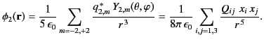 |
(362) |
It follows, from the previous analysis, that the first three terms in the multipole expansion, (340), can be written
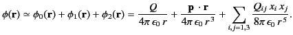 |
(363) |
Moreover, at sufficiently large
, these are always the dominant terms in the expansion.
Next: Axisymmetric Charge Distributions
Up: Potential Theory
Previous: Poisson's Equation in Spherical
Richard Fitzpatrick
2014-06-27