


Next: Spherical Wave Expansion of
Up: Multipole Expansion
Previous: Sources of Multipole Radiation
As an illustration of the use of a multipole expansion for a source whose
dimensions are comparable to a wavelength, consider the radiation
from a linear centre-fed antenna. We assume that the antenna runs along the
 -axis, and extends from
  to
to  . The current flowing
along the antenna vanishes at the end points, and is an even function
of
. Thus, we can write
. The current flowing
along the antenna vanishes at the end points, and is an even function
of
. Thus, we can write
 |
(1547) |
where  . Because the current flows radially,
 . Furthermore, there is no
intrinsic magnetization. Thus, according to Equations (1547)-(1548), all
of the magnetic multipole coefficients,
. Furthermore, there is no
intrinsic magnetization. Thus, according to Equations (1547)-(1548), all
of the magnetic multipole coefficients,  , vanish. In order
to calculate the electric multipole coefficients,
, vanish. In order
to calculate the electric multipole coefficients,  , we need
expressions for the charge and current densities. In spherical
polar coordinates, the current density
, we need
expressions for the charge and current densities. In spherical
polar coordinates, the current density  can be written in
the form
can be written in
the form
![$\displaystyle {\bf j}({\bf r}) = \frac{I(r)}{2\pi \,r^{\,2}} \,\left[\delta(\cos\theta-1)-\delta(\cos\theta+1)\right]{\bf e}_r,$](img3250.png) |
(1548) |
for  ,
where the delta functions cause the current to flow only upwards and
downwards along the
-axis. From the continuity
equation (1522), the charge density is given by
,
where the delta functions cause the current to flow only upwards and
downwards along the
-axis. From the continuity
equation (1522), the charge density is given by
![$\displaystyle \rho({\bf r}) = \frac{1}{{\rm i}\,\omega} \frac{d I(r)}{dr} \left[\frac{\delta(\cos\theta-1) -\delta(\cos\theta+1)}{2\pi\, r^{\,2}}\right],$](img3252.png) |
(1549) |
for
.
The above expressions for
and  can be substituted into
Equation (1543) to give
can be substituted into
Equation (1543) to give
The angular integral has the value
![$\displaystyle \oint Y_{lm}^{\,\ast}\left[\delta(\cos\theta-1) -\delta(\cos\thet...
...right]d{\mit\Omega} = 2\pi\,\delta_{m0}\, \left[Y_{l0}(0) - Y_{l0}(\pi)\right],$](img3255.png) |
(1551) |
showing that only  multipoles are generated. This is hardly surprising,
given the cylindrical symmetry of the antenna. The
spherical
harmonics are even (odd) about
multipoles are generated. This is hardly surprising,
given the cylindrical symmetry of the antenna. The
spherical
harmonics are even (odd) about
 for
for  even (odd).
Hence, the only nonvanishing multipoles have
odd, and the angular
integral reduces to
even (odd).
Hence, the only nonvanishing multipoles have
odd, and the angular
integral reduces to
![$\displaystyle \oint Y_{lm}^{\,\ast}\left[\delta(\cos\theta-1) -\delta(\cos\theta+1)\right] d\Omega = \sqrt{4\pi\,(2\,l+1)}.$](img3256.png) |
(1552) |
After some slight rearrangement, Equation (1552)
can be written
 |
(1553) |
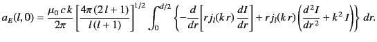
In order to evaluate the above integral, we need to specify the current
 along the antenna. In the absence of radiation, the sinusoidal
time variation at frequency
along the antenna. In the absence of radiation, the sinusoidal
time variation at frequency  implies a sinusoidal space variation
with wavenumber
implies a sinusoidal space variation
with wavenumber
 . However, the emission of radiation
generally modifies the current distribution. The correct current
can only be found be solving a complicated boundary value problem.
For the sake of simplicity, we assume that
is a known function:
specifically,
. However, the emission of radiation
generally modifies the current distribution. The correct current
can only be found be solving a complicated boundary value problem.
For the sake of simplicity, we assume that
is a known function:
specifically,
 |
(1554) |
for  , where
  is the peak current.
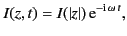
With a sinusoidal
current, the second term in curly brackets in Equation (1555) vanishes. The
first term is a perfect differential. Consequently, Equations (1555)
and (1556) yield
is the peak current.
With a sinusoidal
current, the second term in curly brackets in Equation (1555) vanishes. The
first term is a perfect differential. Consequently, Equations (1555)
and (1556) yield
![$\displaystyle a_E(l, 0) = \frac{\mu_0\, c\, I}{\pi \,d}\left[\frac{4\pi\, (2\,l+1)} {l\,(l+1)}\right]^{1/2} \left(\frac{k\,d}{2}\right)^2\,j_l(k\,d/2),$](img3261.png) |
(1555) |
for
odd.
Let us consider the special cases of a half-wave antenna
(i.e.,  , so that the length of the antenna is
half a wavelength) and a full-wave antenna (i.e.,
, so that the length of the antenna is
half a wavelength) and a full-wave antenna (i.e.,  ). For
these two values of
). For
these two values of  , the
, the
 electric multipole coefficient is tabulated in Table 3, along with the relative
values for
electric multipole coefficient is tabulated in Table 3, along with the relative
values for  and
and  .
It is clear, from the table,
that the coefficients decrease rapidly in magnitude as
increases, and
that higher
coefficients are more important the larger the source
dimensions. However, even for a full-wave antenna, it is generally sufficient
to retain only the
and
coefficients when calculating the angular
distribution of the radiation. It is certainly adequate to keep only
these two harmonics when calculating the total radiated power
(which depends on the sum of the squares of the coefficients).
.
It is clear, from the table,
that the coefficients decrease rapidly in magnitude as
increases, and
that higher
coefficients are more important the larger the source
dimensions. However, even for a full-wave antenna, it is generally sufficient
to retain only the
and
coefficients when calculating the angular
distribution of the radiation. It is certainly adequate to keep only
these two harmonics when calculating the total radiated power
(which depends on the sum of the squares of the coefficients).
Table 3:
The first few electric multipole coefficients for a half-wave
and a full-wave antenna.
|
|
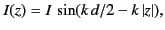
In the radiation zone, the multipole fields (1479)-(1480) reduce to
where use has been made of the asymptotic form (1432).
The time-averaged power radiated per unit solid angle is given by
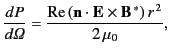 |
(1558) |
or
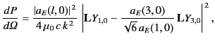
![$\displaystyle \frac{dP}{d{\mit \Omega}} = \frac{1}{2\,\mu_0\, c \, k^{\,2}}\lef...
...,m)\,{\bf X}_{lm} +a_M(l,m)\,{\bf n}\times{\bf X}_{lm}\right]\right\vert^{\,2}.$](img3276.png) |
(1559) |
Retaining only the
and
electric multipole coefficients, the
angular distribution of the radiation from the antenna takes the form
 |
(1560) |
where use has been made of Equation (1476).
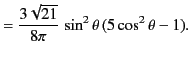
The various factors in the absolute square are
With these angular factors, Equation (1561) becomes
 |
(1564) |
where  equals 1 for a half-wave antenna, and
  for a
full-wave antenna. The coefficient in front of
for a
full-wave antenna. The coefficient in front of
 is
is  and
and  for the half-wave and full-wave antenna, respectively.
It turns out that the radiation pattern obtained from the
two-term multipole expansion specified in the previous equation is
almost indistinguishable from the exact result for the case of a half-wave
antenna. For the case of a full-wave antenna, the two-term expansion
yields a radiation pattern that differs from the exact result by less
than 5 percent.
for the half-wave and full-wave antenna, respectively.
It turns out that the radiation pattern obtained from the
two-term multipole expansion specified in the previous equation is
almost indistinguishable from the exact result for the case of a half-wave
antenna. For the case of a full-wave antenna, the two-term expansion
yields a radiation pattern that differs from the exact result by less
than 5 percent.
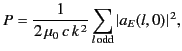
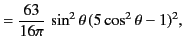
The total power radiated by the antenna is
 |
(1565) |
where use has been made of Equation (1500). It is evident from Table 3
that a two-term multipole expansion gives an accurate expression for the
power radiated by both a half-wave and a full-wave antenna. In fact, a
one-term multipole expansion gives a fairly accurate result for the
case of a half-wave antenna.
It is clear, from the previous analysis, that the multipole expansion converges
rapidly when the source dimensions are of order the wavelength of the radiation. It is also clear that if the source dimensions are much less than
the wavelength then the multipole expansion is likely to be completely
dominated by the term corresponding to the lowest value of
.
Next: Spherical Wave Expansion of
Up: Multipole Expansion
Previous: Sources of Multipole Radiation
Richard Fitzpatrick
2014-06-27
![$\displaystyle \simeq \frac{{\rm e}^{\,{\rm i}\,(k\,r -\omega \,t)}}{k\,r} \sum_...
...+1} \left[ a_E(l,m)\,{\bf X}_{lm}+ a_M(l,m) \,{\bf n}\times{\bf X}_{lm}\right],$](img3273.png)

![$\displaystyle =\frac{\mu_0\, c\,k^{\,2}}{2\pi\sqrt{l\,(l+1)}} \int_0^{d/2}\left...
...(k\,r)\,I(r) -\frac{1}{k} \frac{dI(r)}{dr} \frac{d[r\,j_l(k\,r)]}{dr}\right\}dr$](img3253.png)
![$\displaystyle \oint Y_{lm}^{\,\ast}\left[\delta(\cos\theta-1) -\delta(\cos\theta+1)\right]d{\mit\Omega}.$](img3254.png)