Next: Exercises
Up: Maxwell's Equations
Previous: Electromagnetic Energy Conservation
Electromagnetic Momentum Conservation
Let  be the density of electromagnetic momentum directed parallel to the
  th Cartesian axis. (Here,
  corresponds to the
  -axis,
  to
the
to
the  -axis, and
  to the
  -axis.) Furthermore, let
 be the flux of such momentum.
We would expect the conservation equation for electromagnetic momentum directed parallel to the
th Cartesian axis to take the form
be the flux of such momentum.
We would expect the conservation equation for electromagnetic momentum directed parallel to the
th Cartesian axis to take the form
 |
(111) |
where the subscript
denotes a component of a vector parallel to the
th Cartesian axis. The term on the right-hand side is the
rate per unit volume at which electromagnetic fields gain momentum parallel to the
th Cartesian axis via interaction with matter.
Thus, the term is minus the rate at which matter gains momentum parallel to the
th Cartesian axis via interaction with
electromagnetic fields. In other words, the term is minus the
th component of the force per unit volume exerted on matter
by electromagnetic fields. [See Equation (10).]
Equation (111) can be generalized to give
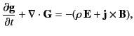 |
(112) |
where  is the electromagnetic momentum density (the
th Cartesian component of
is thus
), and
is the electromagnetic momentum density (the
th Cartesian component of
is thus
), and  is a tensor (see Section 12.5) whose Cartesian components
 , where
  is a unit vector parallel to the
  th Cartesian axis, specify the flux of electromagnetic momentum parallel to the
th Cartesian
axis across a plane surface whose normal is parallel to the
th Cartesian axis.
Let us attempt to derive an expression of the form (112) from Maxwell's equations.
th Cartesian axis, specify the flux of electromagnetic momentum parallel to the
th Cartesian
axis across a plane surface whose normal is parallel to the
th Cartesian axis.
Let us attempt to derive an expression of the form (112) from Maxwell's equations.
Maxwell's equations are as follows:
We can take the vector product of Equation (116) divided by  with
with  , and rearrange, to give
 |
(117) |
Next, we can take the vector product of  with Equation (115) times
 ,
rearrange, and add the result to the previous equation. We obtain
,
rearrange, and add the result to the previous equation. We obtain
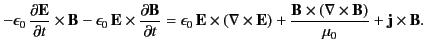 |
(118) |
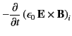
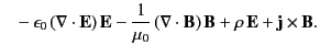
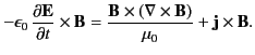
Making use of Equations (113) and (114), we get
Now,
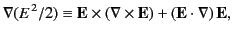 |
(120) |
with a similar equation for
. Hence, Equation (119)
can be written
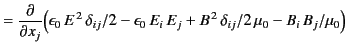
Finally, when written in terms of components, the above equation becomes
because
![$ [(\nabla\cdot{\bf E})\,{\bf E}]_i \equiv (\partial E_j/\partial x_j)\,E_i$](img305.png) ,
and
,
and
![$ [({\bf E}\cdot\nabla)\,{\bf E}]_i \equiv E_j\,(\partial E_i/\partial x_j)$](img306.png) .
Here,
.
Here,  corresponds to
,
corresponds to
,  to
, and
to
, and  to
. Furthermore,
to
. Furthermore,
 is a Kronecker delta symbol (i.e.,
 if
if  , and
, and
 otherwise). Finally, we are making use of the Einstein summation convention (that repeated indices are summed from 1 to 3).
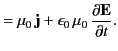
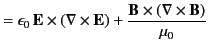
Comparing the previous expression with Equation (112), we conclude that
the momentum density of electromagnetic fields takes the form
otherwise). Finally, we are making use of the Einstein summation convention (that repeated indices are summed from 1 to 3).
Comparing the previous expression with Equation (112), we conclude that
the momentum density of electromagnetic fields takes the form
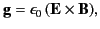 |
(123) |
whereas the corresponding
momentum flux tensor has the Cartesian components
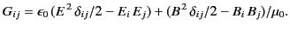 |
(124) |
The momentum conservation equation, (112), is sometimes written
 |
(125) |
where
 |
(126) |
is called the Maxwell stress tensor.
Next: Exercises
Up: Maxwell's Equations
Previous: Electromagnetic Energy Conservation
Richard Fitzpatrick
2014-06-27

![$\displaystyle \phantom{=} +\frac{1}{\mu_0}\left[\nabla(B^{\,2}/2) - (\nabla\cdot {\bf B})\,{\bf B} - ({\bf B}\cdot\nabla)\,{\bf B}\right]$](img300.png)