


Next: Thomson Scattering
Up: Radiation and Scattering
Previous: Antenna Directivity and Effective
Consider a linear array of  half-wave antennas arranged
along the
half-wave antennas arranged
along the  -axis with a uniform spacing
 .
Suppose that each
antenna is aligned along the
.
Suppose that each
antenna is aligned along the  -axis, and also that all
antennas are driven in phase. Let one end of
the array coincide with the origin. The field produced in
the radiation zone by the end-most antenna is given by [see Equation (1231)]
-axis, and also that all
antennas are driven in phase. Let one end of
the array coincide with the origin. The field produced in
the radiation zone by the end-most antenna is given by [see Equation (1231)]
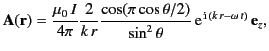 |
(1263) |
where  is the peak current flowing in each antenna.
The fields produced at a given point in the radiation zone by successive
elements of the array differ in phase by an amount
is the peak current flowing in each antenna.
The fields produced at a given point in the radiation zone by successive
elements of the array differ in phase by an amount
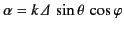 . Here,
  ,
,  ,
,  are conventional
spherical polar coordinates.
Thus, the total field is given by
are conventional
spherical polar coordinates.
Thus, the total field is given by
![$\displaystyle {\bf A}({\bf r}) =\frac{\mu_0\,I}{4\pi} \frac{2 }{k\,r} \frac{\co...
...\,{\rm i}\,\alpha}\right]\, {\rm e}^{\,{\rm i}\,(k\,r-\omega\, t)} \,{\bf e}_z.$](img2693.png) |
(1264) |
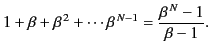
The series in square brackets is a geometric progression in
 , the sum of which takes the value
 |
(1265) |
Thus, the term in square brackets becomes
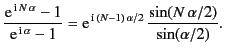 |
(1266) |
It follows from Equation (1232) that the radiation pattern due to the
array takes the form
![$\displaystyle \frac{d P}{d{\mit \Omega}}=\left[\frac{\mu_0\,c\,I^{\,2}}{8\pi^2}...
...in^2\theta} \right] \left[\frac{\sin^2(N\,\alpha/2)}{\sin^2(\alpha /2)}\right].$](img2697.png) |
(1267) |
We can think of this formula as the product of the
two factors in large parentheses. The first is just the standard
radiation pattern of a half-wave antenna. The second arises from the
arrangement of the array. If we retained the same array, but replaced
the elements by something other than half-wave antennas, then the first
factor would change, but not the second. If we changed the array, but not
the elements, then the second factor would change, but the first would
remain the same. Thus, the radiation pattern as the product of two independent factors, the element function, and the array
function. This independence follows from the Fraunhofer
approximation, (1221), which justifies the linear phase shifts of Equation (1222).
The array function in the present case is
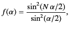 |
(1268) |
where
 |
(1269) |
The function  has nulls whenever the numerator vanishes:
that is, whenever
has nulls whenever the numerator vanishes:
that is, whenever
 |
(1270) |
However, when
 , the denominator also vanishes, and
the l'Hôpital limit is easily seen to be
, the denominator also vanishes, and
the l'Hôpital limit is easily seen to be
 . These limits are known as the principal maxima of the function.
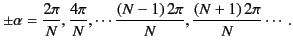
Secondary maxima occur approximately at the maxima of the numerator:
that is, at
. These limits are known as the principal maxima of the function.
Secondary maxima occur approximately at the maxima of the numerator:
that is, at
 |
(1271) |
There are  secondary maxima between successive principal maxima.
Now, the maximum possible value of  is
is
 . Thus, when the element spacing
is less
than the wavelength there is only one principal maximum (at
. Thus, when the element spacing
is less
than the wavelength there is only one principal maximum (at  ),
directed perpendicular to the array (i.e., at
),
directed perpendicular to the array (i.e., at
 ). Such a system is called a broadside array.
The secondary maxima of the radiation pattern are called side lobes.
In the direction perpendicular
to the array, all elements contribute in phase, and the intensity
is proportional to the square of the sum of the individual amplitudes.
Thus, the peak intensity for an
element array is
). Such a system is called a broadside array.
The secondary maxima of the radiation pattern are called side lobes.
In the direction perpendicular
to the array, all elements contribute in phase, and the intensity
is proportional to the square of the sum of the individual amplitudes.
Thus, the peak intensity for an
element array is  times the
intensity of a single antenna. The angular half-width of the principle
maximum (in
) is approximately
times the
intensity of a single antenna. The angular half-width of the principle
maximum (in
) is approximately
 . Although the principal lobe clearly gets narrower in
the azimuthal angle
as
increases, the lobe width
in the polar angle
is mainly controlled by the element
function, and is thus little affected by the number of elements.
A radiation pattern which is narrow in one angular dimension, but broad
in the other, is called a fan beam.
. Although the principal lobe clearly gets narrower in
the azimuthal angle
as
increases, the lobe width
in the polar angle
is mainly controlled by the element
function, and is thus little affected by the number of elements.
A radiation pattern which is narrow in one angular dimension, but broad
in the other, is called a fan beam.
Arranging a set of antennas in a regular array has the effect of
taking the azimuthally symmetric radiation pattern of an individual
antenna and concentrating it into some narrow region of azimuthal angle of
extent
 . The net result is that the gain of the
array is larger than that of an individual antenna by a factor of
order
. The net result is that the gain of the
array is larger than that of an individual antenna by a factor of
order
 |
(1272) |
It is clear that the boost factor is of order the linear extent of
the array divided by the wavelength of the emitted radiation. Thus, it
is possible to construct a very high gain antenna by arranging
a large number of low gain antennas in a regular pattern, and driving
them in phase. The optimum spacing between successive elements of the
array is of order the wavelength of the radiation.
A linear array of antenna elements that are spaced
 apart, and driven with alternating phases, has its principal radiation
maximum along
apart, and driven with alternating phases, has its principal radiation
maximum along
 and
and  , because the
field amplitudes now add in phase in the plane of the array.
Such a system is called an
end-fire array. The direction of the principal maximum can be changed
at will by introducing the appropriate phase shift between successive elements
of the array. In fact, it is possible to produce a radar beam that
sweeps around the horizon, without any mechanical motion of the array,
by varying the phase difference between successive elements
of the array electronically.
, because the
field amplitudes now add in phase in the plane of the array.
Such a system is called an
end-fire array. The direction of the principal maximum can be changed
at will by introducing the appropriate phase shift between successive elements
of the array. In fact, it is possible to produce a radar beam that
sweeps around the horizon, without any mechanical motion of the array,
by varying the phase difference between successive elements
of the array electronically.
Next: Thomson Scattering
Up: Radiation and Scattering
Previous: Antenna Directivity and Effective
Richard Fitzpatrick
2014-06-27