


Next: Exercises
Up: Magnetostatic Fields
Previous: Circular Current Loop
Localized Current Distribution
Consider the magnetic field generated by a current distribution that is localized in some relatively small region of space centered on the origin.
From Equation (621), we have
 |
(661) |
Assuming that  , so that our observation point lies well outside the distribution, we can write
 |
(662) |
Thus, the  th Cartesian component of the vector potential has the expansion
 |
(663) |
Consider the integral
 |
(664) |
where
 is a divergence-free [see Equation (618)] localized current distribution, and
 and
and
 are
two well-behaved functions.
Integrating the first term by parts, making use of the fact that
are
two well-behaved functions.
Integrating the first term by parts, making use of the fact that
 as
as
 (because the current distribution
is localized), we obtain
(because the current distribution
is localized), we obtain
![$\displaystyle K=\int\left[-g\,\nabla'\cdot(f\,{\bf j})+g\,{\bf j}\cdot\nabla' f\right]dV'$](img1388.png) |
(665) |
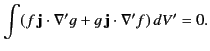
Hence,
![$\displaystyle K = \int\left[-g\,{\bf j}\cdot\nabla' f -g\,f\,\nabla'\cdot{\bf j}+g\,{\bf j}\cdot\nabla' f\right]dV'=0,$](img1389.png) |
(666) |
because
 . Thus, we have proved that
 |
(667) |
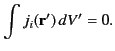
Let  and
and  (where
  is the
th component of
is the
th component of  ). It immediately follows from Equation (668) that
 |
(668) |
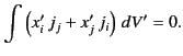
Likewise, if  and
and  then Equation (668) implies that
 |
(669) |
According to Equations (664) and (669),
 |
(670) |
Now,
 |
(671) |
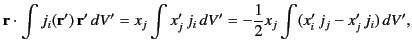
where use has been made of Equation (670), as well as the Einstein summation convention. Thus,
![$\displaystyle {\bf r}\cdot\int j_i\,{\bf r}'\,dV' = -\frac{1}{2}\int \left[({\b...
... = -\frac{1}{2}\left[{\bf r}\times \int ({\bf r}'\times {\bf j})\,dV'\right]_i.$](img1401.png) |
(672) |
Hence, we obtain
 |
(673) |
It is conventional to define the magnetization, or magnetic moment density, as
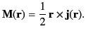 |
(674) |
The integral of this quantity is known as the magnetic moment:
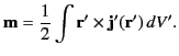 |
(675) |
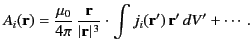
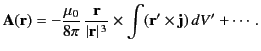
It immediately follows from Equation (674) that the vector potential a long way from a localized current distribution takes the form
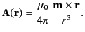 |
(676) |
The corresponding magnetic field is
![$\displaystyle {\bf B}({\bf r}) = \nabla\times {\bf A} = \frac{\mu_0}{4\pi}\left[\frac{3\,({\bf m}\cdot{\bf r})\,{\bf r} -r^{\,2}\,{\bf m}}{r^{\,5}}\right].$](img1406.png) |
(677) |
Thus, we have demonstrated that the magnetic field far from any localized current distribution takes the form of a magnetic
dipole field whose moment is given by the integral (676).
Consider a localized current distribution that consists of a closed planar loop carrying the current  . If
. If  is a
line element of the loop then Equation (676) reduces to
is a
line element of the loop then Equation (676) reduces to
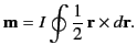 |
(678) |
However,
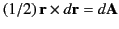 , where
  is a triangular element of vector area defined by the two ends of
and the origin.
Thus, the loop integral gives the total vector area,
is a triangular element of vector area defined by the two ends of
and the origin.
Thus, the loop integral gives the total vector area,  , of the loop. It follows that
 |
(679) |
where  is a unit normal to the loop in the sense determined by the right-hand circulation rule (with the current determining the sense
of circulation). Of course, Equation (680) is identical to Equation (659).
is a unit normal to the loop in the sense determined by the right-hand circulation rule (with the current determining the sense
of circulation). Of course, Equation (680) is identical to Equation (659).
Next: Exercises
Up: Magnetostatic Fields
Previous: Circular Current Loop
Richard Fitzpatrick
2014-06-27