Next: Radiation Losses
Up: Relativity and Electromagnetism
Previous: Accelerated Charges
Let us transform to the inertial frame in which the charge is instantaneously
at rest at the origin at time
 . In this frame,
  ,
so that
,
so that
 and
and  for
events that are sufficiently close to the origin at
that the retarded
charge still appears to travel with a velocity that is small
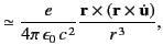
compared to that of light. It follows from the previous section that
for
events that are sufficiently close to the origin at
that the retarded
charge still appears to travel with a velocity that is small
compared to that of light. It follows from the previous section that
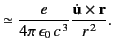
Let us define spherical polar coordinates whose axis points along the
direction of instantaneous
acceleration of the charge.
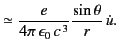
It is easily demonstrated that
These fields are identical to those of a radiating dipole whose axis is
aligned along the direction of instantaneous acceleration. The radial Poynting flux
is given by
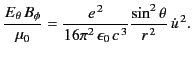 |
(1925) |
We can integrate this expression to obtain the instantaneous
power radiated by the charge
 |
(1926) |
This is known as Larmor's formula. Note that zero net momentum
is carried off by the fields (1925) and (1926).
In order to proceed further, it is necessary to prove two useful theorems.
The first theorem states that if a 4-vector field  satisfies
 |
(1927) |
and if the components of
are non-zero only in a finite
spatial region, then the integral over 3-space,
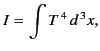 |
(1928) |
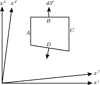
is an invariant. In order to prove this theorem, we need to
use the 4-dimensional analog of Gauss's theorem, which states that
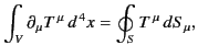 |
(1929) |
where  is an element of the 3-dimensional surface
  bounding the 4-dimensional volume
  . The
particular volume over which the
integration is performed is indicated in Figure 27. The surfaces
. The
particular volume over which the
integration is performed is indicated in Figure 27. The surfaces
 and
and  are chosen so that the spatial components of
vanish on
and
. This is always possible because it is assumed that
the region over which the components of
are non-zero
is of finite extent. The surface
are chosen so that the spatial components of
vanish on
and
. This is always possible because it is assumed that
the region over which the components of
are non-zero
is of finite extent. The surface  is chosen normal to the
  -axis,
whereas the surface
-axis,
whereas the surface  is chosen normal to the
  -axis. Here,
the
-axis. Here,
the  and the
 are coordinates in two arbitrarily
chosen inertial frames. It follows from Equation (1931) that
are coordinates in two arbitrarily
chosen inertial frames. It follows from Equation (1931) that
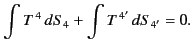 |
(1930) |
Here, we have made use of the fact that
 is a scalar
and, therefore, has the same value in all inertial frames. Because
is a scalar
and, therefore, has the same value in all inertial frames. Because
 and
and
 it follows that
 is an invariant under a Lorentz transformation.
Incidentally, taking the limit in which the two inertial frames are identical, the previous argument also demonstrates that
is an invariant under a Lorentz transformation.
Incidentally, taking the limit in which the two inertial frames are identical, the previous argument also demonstrates that  is constant
in time.
is constant
in time.
Figure 27:
Application of Gauss' theorem.
 |
The second theorem is an extension of the first. Suppose that a 4-tensor
field
 satisfies
 |
(1931) |
and has components which are only non-zero in a finite spatial
region. Let  be a 4-vector whose coefficients do not vary with
position in space-time.
It follows that
be a 4-vector whose coefficients do not vary with
position in space-time.
It follows that
 satisfies Equation (1929). Therefore,
 |
(1932) |
is an invariant. However, we can write
 |
(1933) |
where
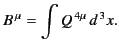 |
(1934) |
It follows from the quotient rule that if
 is an invariant
for arbitrary
then
is an invariant
for arbitrary
then  must transform as a
constant (in time) 4-vector.
must transform as a
constant (in time) 4-vector.
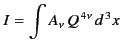
These two theorems enable us to convert differential conservation laws
into integral conservation laws. For instance, in differential form,
the conservation of electrical charge is written
 |
(1935) |
However, from Equation (1932) this immediately implies that
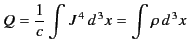 |
(1936) |
is an invariant. In other words, the total electrical charge contained in
space is both constant in time, and the same in all inertial frames.
Suppose that
is the instantaneous rest frame of the charge. Let us
consider the electromagnetic energy tensor
 associated with
all of the radiation emitted by the charge between times
and
associated with
all of the radiation emitted by the charge between times
and  .
According to Equation (1880), this tensor field satisfies
.
According to Equation (1880), this tensor field satisfies
 |
(1937) |
apart from a region of space of measure zero in the vicinity of the charge.
Furthermore, the region of space over which
is non-zero is
clearly finite, because we are only considering the fields emitted by the
charge in a small time interval, and these fields propagate at a
finite velocity. Thus, according to the second theorem,
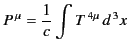 |
(1938) |
is a 4-vector. It follows from Section 12.22 that we can write
 , where
  and
and  are the total
momentum and energy carried off by the radiation emitted between times
and
, respectively. As we have already mentioned,
are the total
momentum and energy carried off by the radiation emitted between times
and
, respectively. As we have already mentioned,
 in the instantaneous rest frame
. Transforming to an
arbitrary inertial frame
in the instantaneous rest frame
. Transforming to an
arbitrary inertial frame
 , in which the instantaneous velocity of the charge is
  ,
we obtain
,
we obtain
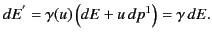 |
(1939) |
However, the time interval over which the radiation is emitted in
is
 . Thus, the instantaneous power radiated by the charge,
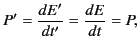 |
(1940) |
is the same in all inertial frames.
We can make use of the fact that the power radiated by an accelerating charge
is Lorentz invariant to find a relativistic generalization of the
Larmor formula, (1928), which is valid in all inertial frames. We expect the
power emitted by the charge to depend only on its 4-velocity and
4-acceleration.
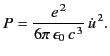
It follows that the Larmor formula can be written in Lorentz invariant form as
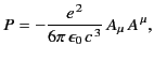 |
(1941) |
because the 4-acceleration takes the form
 in the instantaneous rest frame. In a general inertial
frame,
in the instantaneous rest frame. In a general inertial
frame,
 |
(1942) |
where use has been made of Equation (1726).
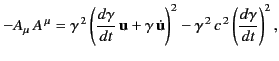
Furthermore, it is easily demonstrated that
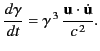 |
(1943) |
It follows, after a little algebra, that the relativistic generalization
of Larmor's formula takes the form
![$\displaystyle P= \frac{e^{\,2}}{6\pi\,\epsilon_0\, c^{\,3}}\, \gamma^{\,6} \left[ \dot{\bf u}^{\,2} - \frac{({\bf u}\times\dot{\bf u})^{\,2}}{c^{\,2}}\right].$](img4075.png) |
(1944) |
Next: Radiation Losses
Up: Relativity and Electromagnetism
Previous: Accelerated Charges
Richard Fitzpatrick
2014-06-27