


Next: Exercises
Up: Wave Propagation in Inhomogeneous
Previous: WKB Reflection Coefficient
In the preceding section, there is a tacit assumption that the square of the
refractive index,
 , is a real function. However, as is apparent from
Equation (1056), this is only the case in the ionosphere as long as
electron collisions are negligible. Let us generalize our analysis to
take electron collisions into account.
In fact, the main effect of electron collisions
is to move the zero of
, is a real function. However, as is apparent from
Equation (1056), this is only the case in the ionosphere as long as
electron collisions are negligible. Let us generalize our analysis to
take electron collisions into account.
In fact, the main effect of electron collisions
is to move the zero of
 a short distance off the real axis
(the distance is relatively short provided that we adopt the
physical ordering
a short distance off the real axis
(the distance is relatively short provided that we adopt the
physical ordering
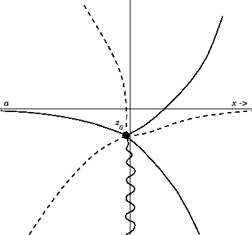
 ). The arrangement of Stokes and anti-Stokes
lines around the new zero point, located at
). The arrangement of Stokes and anti-Stokes
lines around the new zero point, located at
 , is sketched in
Figure 25. Note that electron collisions only significantly modify the
form of
in the immediate vicinity of
the zero point. Thus, sufficiently far away from
in the complex
, is sketched in
Figure 25. Note that electron collisions only significantly modify the
form of
in the immediate vicinity of
the zero point. Thus, sufficiently far away from
in the complex  -plane,
the WKB solutions, as well as the locations of the Stokes and
anti-Stokes lines, are exactly the same as in the preceding section.
-plane,
the WKB solutions, as well as the locations of the Stokes and
anti-Stokes lines, are exactly the same as in the preceding section.
Figure:
The
arrangement of Stokes lines (dashed) and anti-Stokes lines
(solid) in the complex
plane. Also shown is the branch
cut (wavy line).
 |
The WKB solutions (1199) and (1200) are valid all the way along the real
axis, except for a small region close to the origin where electron collisions
significantly modify the form of
. Thus, we can still adopt the
physically reasonable decaying solution (1201) on the positive real axis.
Let us trace this solution in the complex
-plane until we reach the
negative real axis. We can achieve this by moving in a semi-circle in the
upper half-plane. Because we never move out of the region in which the
WKB solutions (1199) and (1200) are valid, we conclude, by analogy with
the preceding section, that the
solution on the negative real axis is given by Equation (1209). Of course, in all
of the WKB solutions the point  must be replaced by the
new zero point
. The new formula for the reflection coefficient,
which is just a straightforward generalization of Equation (1213), is
must be replaced by the
new zero point
. The new formula for the reflection coefficient,
which is just a straightforward generalization of Equation (1213), is
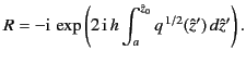 |
(1212) |
This is called the Jeffries connection formula, after H. Jeffries, who
discovered it in 1923. Thus, the general expression for the reflection coefficient
is incredibly simple. We just integrate the WKB solution in the complex
-plane from the phase reference level  to the zero
point, square the result, and multiply by
to the zero
point, square the result, and multiply by  . Note that the path
of integration between
and
does not matter,
because of Cauchy's theorem. Note, also,
that because
. Note that the path
of integration between
and
does not matter,
because of Cauchy's theorem. Note, also,
that because  is, in general, complex along the path of integration,
we no longer have
is, in general, complex along the path of integration,
we no longer have  . In fact, it is easily demonstrated that
 . Thus, when electron collisions are included in the analysis, we
no longer obtain perfect reflection of radio waves from the ionosphere. Instead,
some (small) fraction of the radio energy is absorbed at each reflection
event. This energy is ultimately transferred to the particles in the ionosphere with
which the electrons collide.
. Thus, when electron collisions are included in the analysis, we
no longer obtain perfect reflection of radio waves from the ionosphere. Instead,
some (small) fraction of the radio energy is absorbed at each reflection
event. This energy is ultimately transferred to the particles in the ionosphere with
which the electrons collide.
Next: Exercises
Up: Wave Propagation in Inhomogeneous
Previous: WKB Reflection Coefficient
Richard Fitzpatrick
2014-06-27