Next: Retarded potentials
Up: Time-dependent Maxwell's equations
Previous: Electromagnetic waves
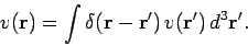
Earlier on in this lecture course, we had to solve Poisson's equation
 |
(475) |
where  is denoted the source function. The potential
  satisfies the boundary condition
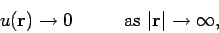 |
(476) |
provided that the source function
is reasonably localized. The solutions to Poisson's equation
are superposable (because the equation is linear). This property is exploited in the Green's
function method of solving this equation. The Green's function
 is the
potential, which satisfies the appropriate boundary conditions,
generated by a unit amplitude
point source located at
is the
potential, which satisfies the appropriate boundary conditions,
generated by a unit amplitude
point source located at  .
Thus,
.
Thus,
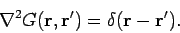 |
(477) |
Any source function can be represented as a weighted sum of point
sources
 |
(478) |
It follows from superposability that the potential generated by the source
can be written as the weighted sum of point source driven
potentials (i.e., Green's functions)
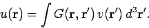 |
(479) |
We found earlier that the Green's function for Poisson's equation is
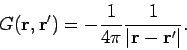 |
(480) |
It follows that the general solution to Eq. (475) is written
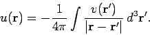 |
(481) |
Note that the point source driven potential (480) is perfectly sensible. It is spherically symmetric
about the source, and falls off smoothly with increasing distance from the source.
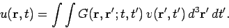
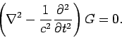
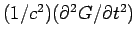
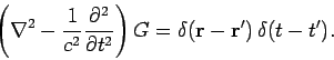
We now need to solve the wave equation
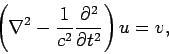 |
(482) |
where  is a time-varying source function. The potential
  satisfies the boundary conditions
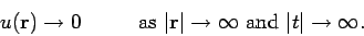 |
(483) |
The solutions to Eq. (482) are superposable (since the equation is linear), so
a Green's function method of solution is again appropriate. The Green's function
 is the potential generated by a point impulse located at
position and applied at time
is the potential generated by a point impulse located at
position and applied at time  . Thus,
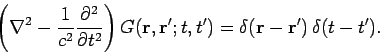 |
(484) |
Of course, the Green's function must satisfy the correct boundary conditions. A general
source can be built up from a weighted sum of point impulses
 |
(485) |
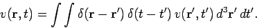
It follows that the potential generated by can be written as the weighted
sum of point impulse driven potentials
 |
(486) |
So, how do we find the Green's function?
Consider
 |
(487) |
where  is a general scalar function. Let us try to prove the following theorem:
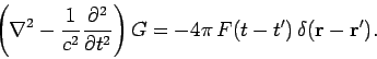 |
(488) |
At a general point,
 , the above expression reduces to
 |
(489) |
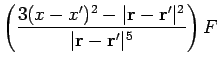
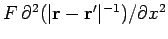
So, we basically have to show that  is a valid solution of the free space
wave equation.
We can easily show that
is a valid solution of the free space
wave equation.
We can easily show that
 |
(490) |
It follows by simple differentiation that
where
 . We can derive analogous equations for
 and
and
 .
Thus,
.
Thus,
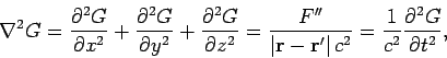 |
(492) |
giving
 |
(493) |
which is the desired result. Consider, now, the region around
 . It is
clear from Eq. (491) that the dominant term on the right-hand
side as
. It is
clear from Eq. (491) that the dominant term on the right-hand
side as
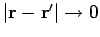 is
the first one, which is essentially
is
the first one, which is essentially
 .
It is also clear that
.
It is also clear that
 is negligible compared to this term.
Thus, as
we find
that
is negligible compared to this term.
Thus, as
we find
that
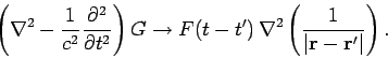 |
(494) |
However, according to Eqs. (477) and (480)
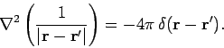 |
(495) |
We conclude that
 |
(496) |
which is the desired result.
Let us now make the special choice
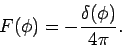 |
(497) |
It follows from Eq. (496) that
 |
(498) |
Thus,
 |
(499) |
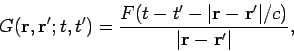
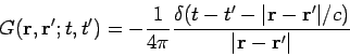
is the Green's function for the driven wave equation (482).
The time-dependent Green's function (499) is the same as the steady-state Green's function
(480), apart from the delta-function appearing in the former. What does this delta-function do?
Well, consider an observer at point  . Because of the delta-function, our observer
only measures a non-zero potential at one particular time
. Because of the delta-function, our observer
only measures a non-zero potential at one particular time
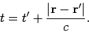 |
(500) |
It is clear that this is the time the impulse was applied at position  (i.e., )
plus the time taken for a light signal to travel between points and
. At time
(i.e., )
plus the time taken for a light signal to travel between points and
. At time  , the locus of all the points at which the potential is non-zero
is
, the locus of all the points at which the potential is non-zero
is
 |
(501) |
In other words, it is a sphere centred on whose radius is the distance traveled by
light in the time interval since the impulse was applied at position .
Thus, the Green's function (499) describes a spherical wave which emanates from position
at time and propagates at the speed of light. The amplitude of the wave
is inversely proportional to the distance from the source.
Next: Retarded potentials
Up: Time-dependent Maxwell's equations
Previous: Electromagnetic waves
Richard Fitzpatrick
2006-02-02