Next: Hamilton's Equations
Up: Hamiltonian Dynamics
Previous: Hamilton's Principle
Suppose that we have a dynamical system described by two generalized
coordinates,  and
and  . Suppose, further, that and are
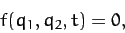
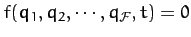
not independent variables. In other words, and are connected
via some constraint equation of the form
. Suppose, further, that and are
not independent variables. In other words, and are connected
via some constraint equation of the form
 |
(714) |
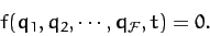
where  is some function of three variables.
This type of constraint is called a holonomic. [A general
holonomic constraint is of the form
is some function of three variables.
This type of constraint is called a holonomic. [A general
holonomic constraint is of the form
 .]
Let
.]
Let
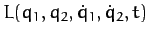 be the Lagrangian.
How do we write the Lagrangian equations of motion of the system?
be the Lagrangian.
How do we write the Lagrangian equations of motion of the system?
Well, according to Hamilton's principle,
![\begin{displaymath}
\delta\int_{t_1}^{t_2} L\,dt = \int_{t_1}^{t_2}\left\{\left[...
... L}{\partial \dot{q}_2}\right)\right]\delta q_2 \right\} dt=0.
\end{displaymath}](img1798.png) |
(715) |
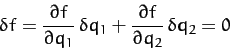
However, at any given instant in time,  and
and  are not independent. Indeed,
Equation (714) yields
are not independent. Indeed,
Equation (714) yields
 |
(716) |
at a fixed time. Eliminating from Equation (715), we obtain
![\begin{displaymath}
\int_{t_1}^{t_2}\left\{\left[
\frac{\partial L}{\partial q_1...
...ht]\frac{1}{\partial f/\partial q_2}\right\} \delta q_1\,dt=0.
\end{displaymath}](img1802.png) |
(717) |
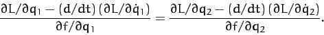
This equation must be satisfied for all possible perturbations  , which implies that the term enclosed in curly brackets is zero.
Hence, we obtain
, which implies that the term enclosed in curly brackets is zero.
Hence, we obtain
 |
(718) |
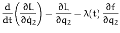
One obvious way in which we can solve this equation is to separately set both sides
equal to the same function of time, which
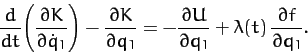
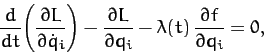
we shall denote  . It follows that the Lagrangian equations of
motion of the system can be written
. It follows that the Lagrangian equations of
motion of the system can be written
In principle, the above two equations can be solved, together with the constraint equation (714), to give  ,
,  , and the
so-called Lagrange multiplier
, and the
so-called Lagrange multiplier  .
Equation (719) can be rewritten
.
Equation (719) can be rewritten
 |
(721) |
Now, the generalized force conjugate to
the generalized coordinate is [see Equation (599)]
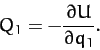 |
(722) |
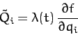
By analogy, it seems clear from Equation (721) that the generalized constraint force [i.e., the generalized force responsible for maintaining the constraint
(714)] conjugate to takes the form
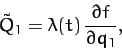 |
(723) |
with a similar expression for the generalized constraint force conjugate to .
Suppose, now, that we have a dynamical system described by  generalized coordinates
  , for
, for  , which is subject to the
holonomic constraint
, which is subject to the
holonomic constraint
 |
(724) |
A simple extension of above analysis yields following the Lagrangian equations of motion of the
system,
 |
(725) |
for . As before,
 |
(726) |
is the generalized constraint force conjugate to .
Finally, the generalization to multiple holonomic constraints is straightforward.
Figure 36:
A cylinder rolling down an inclined plane.
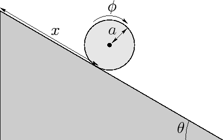 |
Consider the following example. A cylinder of radius  rolls without slipping down a plane
inclined at an angle
rolls without slipping down a plane
inclined at an angle  to the horizontal. Let
  represent the downward displacement of the center of mass of the cylinder parallel to the surface of the plane, and let
  represent the angle of rotation of the cylinder about
its symmetry axis. The fact that the cylinder is rolling without slipping
implies that and are interrelated via the well-known constraint
represent the angle of rotation of the cylinder about
its symmetry axis. The fact that the cylinder is rolling without slipping
implies that and are interrelated via the well-known constraint
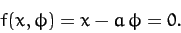 |
(727) |
The Lagrangian of the cylinder takes the form
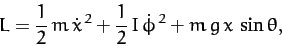 |
(728) |
where  is the cylinder's mass,
  its moment of inertia, and
  the acceleration due to gravity.
Note that
 and
and
 . Hence,
Equation (725) yields the following Lagrangian equations of motion:
. Hence,
Equation (725) yields the following Lagrangian equations of motion:
Equations (727), (729), and (730) can be solved to
give
The generalized constraint force conjugate to is
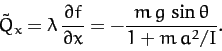 |
(734) |
This represents the frictional force acting parallel to the plane which
impedes the downward acceleration of the cylinder, causing it to be less than the standard value
 . The
generalized constraint force conjugate to is
. The
generalized constraint force conjugate to is
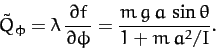 |
(735) |
This represents the frictional torque acting on the cylinder which forces the
cylinder to rotate in such a manner that the constraint (727) is
always satisfied.
Consider a second example. A bead of mass slides without friction
on a vertical circular hoop of radius . Let  be the
radial coordinate of the bead, and let be its
angular coordinate, with the lowest point on the hoop corresponding
to
be the
radial coordinate of the bead, and let be its
angular coordinate, with the lowest point on the hoop corresponding
to  . Both coordinates are measured relative to the
center of the hoop. Now, the bead is constrained to slide along the wire, which implies that
. Both coordinates are measured relative to the
center of the hoop. Now, the bead is constrained to slide along the wire, which implies that
 |
(736) |
Note that
 and
and
 .
The Lagrangian of the system takes the form
.
The Lagrangian of the system takes the form
 |
(737) |
Hence, according to Equation (725), the Lagrangian equations of motion
of the system are written
The second of these equations can be integrated (by multiplying by  ), subject to the constraint (736), to give
 |
(740) |
where  is a constant. Let
  be the tangential velocity of the
bead at the bottom of the hoop (i.e., at ). It follows that
be the tangential velocity of the
bead at the bottom of the hoop (i.e., at ). It follows that
 |
(741) |
Equations (736), (738), and (741) can be combined to give
 |
(742) |
Finally, the constraint force conjugate to is given by
 |
(743) |
This represents the radial reaction exerted on the bead by the hoop. Of course,
there is no constraint force conjugate to (since
) because the bead slides without friction.
Next: Hamilton's Equations
Up: Hamiltonian Dynamics
Previous: Hamilton's Principle
Richard Fitzpatrick
2011-03-31