


Next: Projectile Motion with Air
Up: Multi-Dimensional Motion
Previous: Introduction
Motion in a Two-Dimensional Harmonic Potential
Consider a particle of mass  moving in
the two-dimensional harmonic potential
moving in
the two-dimensional harmonic potential
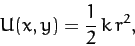 |
(154) |
where
 , and
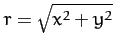
, and  . It follows that the particle is subject to
a force,
. It follows that the particle is subject to
a force,
 |
(155) |
which always points towards the origin, and whose magnitude increases linearly with
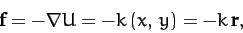
increasing distance from the origin. According to Newton's second law, the
equation of motion of the particle is
 |
(156) |
When written in component form, the above equation reduces to
where
 .
.
Since Equations (157) and (158) are both simple harmonic equations,
we can immediately write their general solutions:
Here,  ,
,  ,
,  , and
, and  are arbitrary constants of integration. We can simplify the above equations slightly by shifting the
origin of time (which is, after all, arbitrary): i.e.,
are arbitrary constants of integration. We can simplify the above equations slightly by shifting the
origin of time (which is, after all, arbitrary): i.e.,
 |
(161) |
Hence, we obtain
where
 .
Note that the motion is clearly periodic in time, with period
.
Note that the motion is clearly periodic in time, with period
 .
Thus, the particle must trace out some closed trajectory in the
.
Thus, the particle must trace out some closed trajectory in the
 -
- plane.
The question, now, is what does this
trajectory look like as a function of
the relative phase-shift,
plane.
The question, now, is what does this
trajectory look like as a function of
the relative phase-shift,  , between the oscillations in the
- and -directions?
, between the oscillations in the
- and -directions?
Using standard trigonometry, we can write Equation (163)
in the form
![\begin{displaymath}
y = B\left[\cos(\omega_0\,t')\,\cos{\mit\Delta} + \sin(\omega_0\,t')\,\sin{\mit\Delta}\right].
\end{displaymath}](img545.png) |
(164) |
Hence, using Equation (162), we obtain
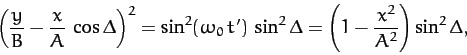 |
(165) |
which simplifies to give
 |
(166) |
Unfortunately, the above equation is not immediately recognizable as being
the equation of any particular geometric curve: e.g., a circle, an ellipse, or
a parabola, etc.
Perhaps our problem is that we are using the wrong coordinates.
Suppose that we rotate our coordinate axes about the  -axis by an
angle
-axis by an
angle  , as illustrated in Figure A.100. According to Equations (A.1277) and (A.1278), our old coordinates (, ) are related to our new coordinates
(
, as illustrated in Figure A.100. According to Equations (A.1277) and (A.1278), our old coordinates (, ) are related to our new coordinates
( ,
,  ) via
) via
Let us see whether Equation (166) takes a simpler form when expressed
in terms of our new coordinates. Equations (166)-(168)
yield
We can simplify the above equation by setting the term involving  to
zero. Hence,
to
zero. Hence,
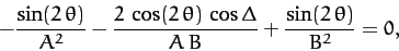 |
(170) |
where we have made use of some simple trigonometric identities. Thus, the term disappears when takes the special value
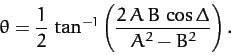 |
(171) |
In this case, Equation (169) reduces to
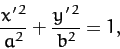 |
(172) |
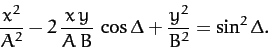
where
Of course, we immediately recognize Equation (172) as the equation of
an ellipse, centered on the origin, whose major and minor axes are aligned along the
- and -axes, and whose major and minor radii are  and
and  ,
respectively (assuming that
,
respectively (assuming that  ).
).
We conclude that, in general, a particle of mass moving in the two-dimensional harmonic potential (154) executes a closed elliptical
orbit (which is not necessarily aligned along the - and -axes), centered on the origin, with
period
, where
.
Figure 10:
Trajectories in a two-dimensional harmonic oscillator potential.
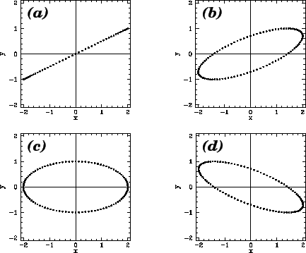 |
Figure 10 shows some example trajectories calculated for  ,
,  , and
the following values of the phase difference, : (a)
, and
the following values of the phase difference, : (a)
 ; (b)
; (b)
 ; (c)
; (c)
 ;
(d)
;
(d)
 . Note that when
the
trajectory degenerates into a straight-line (which can be thought of as an
ellipse whose minor radius is zero).
. Note that when
the
trajectory degenerates into a straight-line (which can be thought of as an
ellipse whose minor radius is zero).
Perhaps, the main lesson to be learned from the above study of two-dimensional
motion in a harmonic potential is that comparatively simple patterns of
motion can be made to look complicated when expressed
in terms of ill-chosen coordinates.
Next: Projectile Motion with Air
Up: Multi-Dimensional Motion
Previous: Introduction
Richard Fitzpatrick
2011-03-31
![$\displaystyle \frac{1}{\sin^2{\mit\Delta}}\left[\frac{\cos^2\theta}{A^2} - \fra...
...s\theta\,\sin\theta\,\cos{\mit\Delta}}{A\,B} + \frac{\sin^2\theta}{B^2}\right],$](img562.png)
![$\displaystyle \frac{1}{\sin^2{\mit\Delta}}\left[\frac{\sin^2\theta}{A^2} +\frac...
...s\theta\,\sin\theta\,\cos{\mit\Delta}}{A\,B} + \frac{\cos^2\theta}{B^2}\right].$](img564.png)
![$\displaystyle x'^{\,2}\left[\frac{\cos^2\theta}{A^2} - \frac{2\,\cos\theta\,\sin\theta\,\cos{\mit\Delta}}{A\,B} + \frac{\sin^2\theta}{B^2}\right]$](img553.png)
![$\displaystyle + y'^{\,2}\left[\frac{\sin^2\theta}{A^2} +\frac{2\,\cos\theta\,\sin\theta\,\cos{\mit\Delta}}{A\,B} + \frac{\cos^2\theta}{B^2}\right]$](img554.png)
![$\displaystyle +x' \,y'\left[-\frac{2\,\sin\theta\,\cos\theta}{A^2} + \frac{2\,(...
...\theta)\,\cos{\mit\Delta}}{A\,B} + \frac{2\,\cos\theta\,\sin\theta}{B^2}\right]$](img555.png)