


Next: Damped Oscillatory Motion
Up: One-Dimensional Motion
Previous: Velocity Dependent Forces
Consider the motion of a point particle of mass  which is
slightly displaced from a stable equilibrium point at
which is
slightly displaced from a stable equilibrium point at  .
Suppose that the particle is moving in the conservative force-field
.
Suppose that the particle is moving in the conservative force-field  . According to the analysis of Section 3.2, in order for to be a stable equilibrium point
we require both
. According to the analysis of Section 3.2, in order for to be a stable equilibrium point
we require both
 |
(72) |
and
 |
(73) |
Now, our particle obeys Newton's second law of motion,
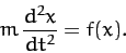 |
(74) |
Let us assume that it always stays fairly close to its equilibrium
point. In this case, to a good approximation, we can represent
via a truncated Taylor expansion about this point. In other words,
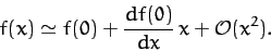 |
(75) |
However, according to (72) and (73), the above
expression can be written
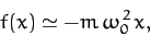 |
(76) |
where
 .
Hence, we conclude that our particle satisfies the following approximate
equation of motion,
.
Hence, we conclude that our particle satisfies the following approximate
equation of motion,
 |
(77) |
provided that it does not stray too far from its equilibrium point: i.e.,
provided  does not become too large.
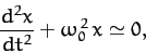
Equation (77) is called the simple harmonic equation, and
governs the motion of all one-dimensional conservative systems which are slightly
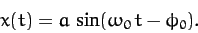
perturbed from some stable equilibrium state. The solution of Equation (77)
is well-known:
 |
(78) |
The pattern of motion described by above expression,
which is called simple harmonic motion,
is periodic in time, with repetition period
 , and oscillates between
  . Here,
  is called the amplitude of the motion. The parameter
  ,
known as the phase angle,
simply shifts the pattern of motion backward and forward in time.
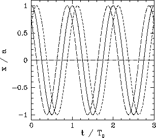
Figure 4 shows some examples of simple harmonic motion.
Here,
,
known as the phase angle,
simply shifts the pattern of motion backward and forward in time.
Figure 4 shows some examples of simple harmonic motion.
Here,  ,
,  , and
, and  correspond to the
solid, short-dashed, and long-dashed curves, respectively.
correspond to the
solid, short-dashed, and long-dashed curves, respectively.
Note that the frequency,  --and, hence, the period,
  --of
simple harmonic motion is determined by the parameters appearing in the simple harmonic equation,
(77). However, the amplitude, , and the phase angle, ,
are the two integration constants of this second-order ordinary differential
equation, and are, thus, determined by the initial conditions: i.e., by the particle's initial displacement and velocity.
--of
simple harmonic motion is determined by the parameters appearing in the simple harmonic equation,
(77). However, the amplitude, , and the phase angle, ,
are the two integration constants of this second-order ordinary differential
equation, and are, thus, determined by the initial conditions: i.e., by the particle's initial displacement and velocity.
Figure 4:
Simple harmonic motion.
 |
Now, from Equations (45) and (76), the potential
energy of our particle at position  is approximately
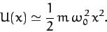 |
(79) |
Hence, the total energy is written
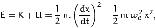 |
(80) |
giving
 |
(81) |
where use has been made of Equation (78), and the trigonometric
identity
 . Note that the
total energy is constant in time, as is to be expected for a
conservative system, and is proportional to the amplitude squared
of the motion.
. Note that the
total energy is constant in time, as is to be expected for a
conservative system, and is proportional to the amplitude squared
of the motion.
Next: Damped Oscillatory Motion
Up: One-Dimensional Motion
Previous: Velocity Dependent Forces
Richard Fitzpatrick
2011-03-31