Next: Roche Radius
Up: Gravitational Potential Theory
Previous: McCullough's Formula
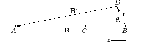
Consider two point masses,  and
and  , executing circular orbits
about their common center of mass,
, executing circular orbits
about their common center of mass,  , with angular
velocity
, with angular
velocity  . Let
. Let  be the distance between
the masses, and
be the distance between
the masses, and  the distance between point and mass --see Figure 41.
We know, from Section 6.3, that
the distance between point and mass --see Figure 41.
We know, from Section 6.3, that
 |
(927) |
and
 |
(928) |
where  .
.
Figure 41:
Two orbiting masses.
 |
Let us transform to a non-inertial frame of reference which rotates, about an axis perpendicular to the orbital plane and passing through , at
the angular velocity . In this reference frame, both masses appear to be stationary. Consider mass . In the rotating frame, this mass experiences
a gravitational acceleration
 |
(929) |
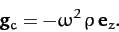
directed toward the center of mass, and a centrifugal acceleration (see Chapter 7)
 |
(930) |
directed away from the center of mass.
However, it is easily demonstrated, using Equations (927) and (928), that
 |
(931) |
In other words, the gravitational and centrifugal accelerations
balance, as must be the case if mass is to remain stationary in the
rotating frame. Let us investigate how this balance is affected if the masses and
have finite spatial extents.
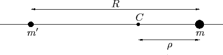
Let the center of the mass distribution lie at  , the center of the
mass distribution at B, and the center of mass at --see Figure 42. We wish to calculate the centrifugal and gravitational
accelerations at some point
, the center of the
mass distribution at B, and the center of mass at --see Figure 42. We wish to calculate the centrifugal and gravitational
accelerations at some point  in the vicinity of point
  . It is
convenient to adopt spherical coordinates, centered on point ,
and aligned such that the
. It is
convenient to adopt spherical coordinates, centered on point ,
and aligned such that the  -axis coincides with the line
  .
.
Figure 42:
Calculation of tidal forces.
 |
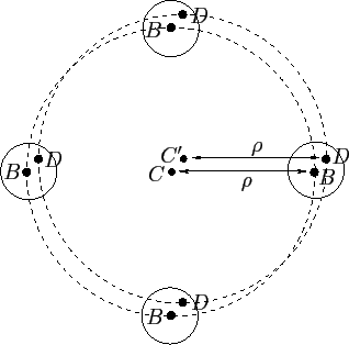
Let us assume that the mass distribution
is orbiting around , but is not rotating about
an axis passing through its center, in order to
exclude rotational flattening from our analysis. If this is the
case then it is easily seen that each constituent point of executes
circular motion of angular velocity and radius --see Figure 43. Hence, each constituent point experiences the same
centrifugal acceleration: i.e.,
 |
(932) |
It follows that
 |
(933) |
where
 |
(934) |
is the centrifugal potential, and
 . The centrifugal potential
can also be written
. The centrifugal potential
can also be written
 |
(935) |
Figure 43:
The center of the mass distribution orbits about the center of mass in a circle of radius . If the mass distribution is non-rotating then a non-central point must maintain a constant spatial relationship to . It follows that point orbits some point  , which has the same spatial relationship to that has to , in a circle
of radius .
, which has the same spatial relationship to that has to , in a circle
of radius .
 |
The gravitational acceleration at point due to mass is given by
 |
(936) |
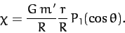
where the gravitational potential takes the form
 |
(937) |
Here,  is the distance between points and . Note that the
gravitational potential generated by the mass distribution is the
same as that generated by an equivalent point mass at , as long
as the distribution is spherically symmetric, which we shall assume to
be the case.
is the distance between points and . Note that the
gravitational potential generated by the mass distribution is the
same as that generated by an equivalent point mass at , as long
as the distribution is spherically symmetric, which we shall assume to
be the case.
Now,
 |
(938) |
where  is the vector
 ,
and
,
and  the vector
 --see Figure 42.
It follows that
--see Figure 42.
It follows that
 |
(939) |
Expanding in powers of  , we obtain
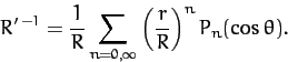 |
(940) |
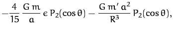
Hence,
![\begin{displaymath}
\Phi' \simeq - \frac{G\,m'}{R}\left[1+ \frac{r}{R}\,P_1(\cos\theta) + \frac{r^2}{R^2}\,P_2(\cos\theta)\right]
\end{displaymath}](img2226.png) |
(941) |
to second-order in .
Adding  and
and  , we obtain
![\begin{displaymath}
\chi+\Phi' \simeq - \frac{G\,m'}{R}\left[1 + \frac{r^2}{R^2}\,P_2(\cos\theta)\right]
\end{displaymath}](img2229.png) |
(942) |
to second-order in . Note that  is the potential
due to the net external force acting on the mass distribution . This
potential is constant up to first-order in , because the first-order
variations in and cancel one another. The
cancellation
is a manifestation of the balance between the centrifugal and gravitational
accelerations in the equivalent point mass problem discussed above. However, this balance
is only exact at the center of the mass distribution . Away from the
center, the centrifugal acceleration remains constant, whereas
the gravitational acceleration increases with increasing . Hence, at positive , the gravitational
acceleration is larger than the centrifugal, giving rise to a net acceleration
in the
is the potential
due to the net external force acting on the mass distribution . This
potential is constant up to first-order in , because the first-order
variations in and cancel one another. The
cancellation
is a manifestation of the balance between the centrifugal and gravitational
accelerations in the equivalent point mass problem discussed above. However, this balance
is only exact at the center of the mass distribution . Away from the
center, the centrifugal acceleration remains constant, whereas
the gravitational acceleration increases with increasing . Hence, at positive , the gravitational
acceleration is larger than the centrifugal, giving rise to a net acceleration
in the  -direction. Likewise, at negative , the centrifugal acceleration
is larger than the gravitational, giving rise to a net acceleration in the
-direction. Likewise, at negative , the centrifugal acceleration
is larger than the gravitational, giving rise to a net acceleration in the  -direction.
It follows that the mass distribution
is subject to a residual acceleration, represented by the second-order variation in Equation (942), which acts to elongate it along the -axis.
This effect is known as tidal elongation.
-direction.
It follows that the mass distribution
is subject to a residual acceleration, represented by the second-order variation in Equation (942), which acts to elongate it along the -axis.
This effect is known as tidal elongation.
In order to calculate the tidal elongation of the mass distribution we
need to add the potential, , due to the external forces, to
the gravitational potential,  , generated by the distribution itself. Assuming that
the mass distribution is spheroidal with mass , mean radius
, generated by the distribution itself. Assuming that
the mass distribution is spheroidal with mass , mean radius  ,
and ellipticity
,
and ellipticity  , it follows from Equations (901), (911),
and (942) that the total surface potential
is given by
, it follows from Equations (901), (911),
and (942) that the total surface potential
is given by
where we have treated and  as small quantities. As before,
the condition for equilibrium is that the total potential be constant
over the surface of the spheroid. Hence, we obtain
as small quantities. As before,
the condition for equilibrium is that the total potential be constant
over the surface of the spheroid. Hence, we obtain
 |
(944) |
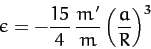
as our prediction for the ellipticity induced in a self-gravitating spherical
mass distribution of total mass and radius by a second mass, ,
which is in a circular orbit of radius about the distribution. Thus, if  is
the maximum radius of the distribution, and
is
the maximum radius of the distribution, and  the minimum radius (see Figure 44), then
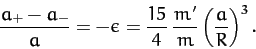 |
(945) |
Figure 44:
Tidal elongation.
 |
Consider the tidal elongation of the Earth due to the Moon. In this
case, we have
 ,
,
 ,
,
 , and
, and
 .
Hence, we calculate that
.
Hence, we calculate that
 , or
, or
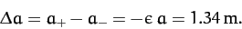 |
(946) |
We, thus, predict that tidal forces due to the Moon cause the
Earth to elongate along the axis joining its center to the Moon by
about  meters. Since water is obviously more fluid than rock
(especially on relatively short time-scales) most of this elongation
takes place in the oceans rather than in the underlying land. Hence,
the oceans rise, relative to the land, in the region of the Earth closest
to the Moon, and also in the region furthest away. Since the Earth
is rotating, whilst the tidal bulge of the oceans remains relatively
stationary, the Moon's tidal force causes the ocean at a given point
on the Earth's surface to rise and fall, by about a meter, twice daily, giving rise to the
phenomenon known as the tides.
meters. Since water is obviously more fluid than rock
(especially on relatively short time-scales) most of this elongation
takes place in the oceans rather than in the underlying land. Hence,
the oceans rise, relative to the land, in the region of the Earth closest
to the Moon, and also in the region furthest away. Since the Earth
is rotating, whilst the tidal bulge of the oceans remains relatively
stationary, the Moon's tidal force causes the ocean at a given point
on the Earth's surface to rise and fall, by about a meter, twice daily, giving rise to the
phenomenon known as the tides.
Consider the tidal elongation of the Earth due to the Sun. In this case,
we have
,
 ,
, and
,
, and
 .
Hence, we calculate that
.
Hence, we calculate that
 , or
, or
 |
(947) |
Thus, the tidal elongation due to the Sun is about half that due to the Moon.
It follows that the tides are particularly high when the Sun, the Earth, and
the Moon lie approximately in a straight-line, so that the tidal effects of the Sun and the Moon reinforce one another. This occurs at a new moon,
or at a full moon. These type of tides are called spring tides (note that
the name has nothing to do with the season). Conversely, the
tides are particularly low when the Sun, the Earth, and the Moon
form a right-angle, so that the tidal effects of the
Sun and the Moon partially cancel one another. These type of tides are called neap tides. Generally
speaking, we would expect two spring tides and two neap tides per month.
In reality, the amplitude of the tides varies significantly from place to place on the Earth's surface, due to the presence of the continents, which impede the flow of the oceanic tidal bulge
around the Earth. Moreover, there is a time-lag of approximately 12 minutes
between the Moon being directly overhead (or directly below) and
high tide, because of the finite inertia of the oceans. Similarly, the time-lag
between a spring tide and a full moon, or a new moon, can be up to 2 days.
Next: Roche Radius
Up: Gravitational Potential Theory
Previous: McCullough's Formula
Richard Fitzpatrick
2011-03-31